Adaptive Modeler is an application for creating agent-based market simulation models for price forecasting of real world market-traded securities such as stocks, ETFs, forex currency pairs, cryptocurrencies, commodities and other markets.

1.1 Agent-based models and financial markets

An agent-based model is a bottom-up simulation of the actions and interactions of multiple individuals and organizations for the purpose of analyzing the (emergent) effects on a system as a whole. An agent-based model of a financial market may consist of a population of agents (representing traders/investors) and a price discovery and clearing mechanism (representing a market).

Agent-based models have shown to be able to explain the behavior of financial markets better than traditional financial models[1]. Conventionally, financial markets have been studied using analytical mathematics and econometric models mostly based on a generalization of supposedly rational market participants (representative rational agent models). However, the empirical features of financial markets can not be fully explained by such models. In reality, market prices are established by a large diversity of boundedly rational (learning) traders with different decision making methods and different characteristics (such as risk preference and time horizon). The complex dynamics of these heterogeneous traders and the resulting price formation require a simulation model consisting of multiple heterogeneous agents and a virtual (artificial) market.

Research has shown that complex behavior as seen in actual markets can emerge from simulations of agents with relatively simple decision rules. Commonly observed empirical features of financial time series (so called “stylized facts” such as fat tails in return distributions and volatility clustering) that have confronted the Efficient Market Hypothesis, have successfully been reproduced in agent-based models[2].

1.2 How Adaptive Modeler uses agent-based models

Adaptive Modeler creates an agent-based market model for a user selected real world security. The model consists of a population of thousands of trader agents, each with their own trading rule, and a virtual market. Adaptive Modeler then evolves this model step by step while feeding it with market prices of the security and (optionally) other variables.

After every received market price, the agents evaluate their trading rule and place buy or sell orders on the Virtual Market where a clearing price is determined and orders are executed. Agents and their trading rules evolve through adaptive genetic programming. Agents with poor performance are being replaced by new agents with a new trading rule that is created by recombining and mutating trading rules of well performing agents.

Self-organization through the evolution of agents and the resulting price dynamics drives the model to learn to recognize and anticipate recurring price patterns while adapting to changing market behavior. Model evolution never ends. When all historical market prices have been processed, the model waits for new price data to become available and then evolves further. The model thus evolves in parallel with the real world market. After every processed price the model generates a forecast for the next bar (or tick) based on the behavior of the Virtual Market. Trading signals are generated based on the forecasts and the user’s trading preferences.

1.3 Adaptive Modeler’s possibilities

Models generate trading signals for a single selected security. Trading signals are based on one-bar-ahead (or one-tick-ahead) price forecasts that are calculated after every received quote bar (or tick). Adaptive Modeler supports quote intervals ranging from 1 millisecond to multiple days as well as variable intervals. The only limiting factors are the available market data and processing speed.

Adaptive Modeler uses evolutionary computation and learns over time. Therefore it is recommended to provide the model with some historical market data. Using at least 1,000 historical quotes is recommended. The more historical data is used, the more opportunity the model has to learn and the more information the user gets on how a model performs during different periods and market regimes. Also, only after a sufficient number of quotes has been processed, statistical significance can be attributed to any demonstrated forecasting accuracy.

Adaptive Modeler is primarily designed for active trading of stocks or stock indices (i.e. using futures or ETFs) with sufficient volatility and small spreads. Because signals tend to switch frequently, Adaptive Modeler is suitable for day trading or swing trading strategies amongst others. Other markets such as forex currency pairs, commodities, Bitcoin or other cryptocurrencies can also be used because in principle Adaptive Modeler can process any sort of time series. In general, the volatility on the used quote interval must be high enough to cover transaction costs (broker commissions, spread and slippage). Otherwise, (simulated) trading performance will be poor even with high forecasting accuracy. For example, it will be more difficult to achieve good performance with a 1-minute interval than with a daily interval because the 1-minute price changes may be too small to cover transaction costs. This means that the break-even forecast accuracy rate for a 1-minute interval is higher than for a daily interval.

Adaptive Modeler provides an extensive set of output data and visualization tools to observe the historical evolution of a model, its current behavior and the accuracy and significance of previous forecasts and trading signals. Also it is possible to simulate trading and to project the likely range of returns under given assumptions. Extensive performance analysis is available to study risk and return measures of simulated trading. However, as for any system that aims to make predictions about the future, there is no guarantee that any demonstrated forecasting success or trading performance will remain the same in the future. Past performance or results implied, shown or otherwise demonstrated by Adaptive Modeler can not guarantee future performance or results. The user should be aware of this and consider the risks and potential rewards of every investment or trading decision on its own merits.

Trading can be simulated according to user customizable trading parameters such as enabling/disabling short positions, close positions at the end of the day, expected spread and slippage, and others.

Adaptive Modeler does not contain built-in support for online market data feeds nor does it contain interfaces for automatic order placement with online brokers. Market data is imported from CSV files using a flexible and intelligent file reader and output data such as forecasts and trading signals can be exported to CSV files for further processing by other applications. Traders are encouraged to supplement Adaptive Modeler’s signals with their own order placement algorithms for actual automated trading.

1.4 Specifications

Some specifications and limitations of the different editions of Adaptive Modeler[3]:

Feature	Evaluation Edition	Standard Edition	Professional Edition
Forecasts and trading signals	delayed [4]	real-time	real-time
Maximum number of agents	5,000	25,000	250,000
Maximum genome size	1,024	4,096	4,096
Maximum genome depth	20	20	unlimited[5]
Maximum bars	20,000	20,000	unlimited [6]
Maximum bars stored[7]	20,000	20,000	100,000
Manual Export (max bars)	500	20,000	100,000
Auto Export	No	No	Yes
Batch Mode (max models)	4[8]	unlimited[9]	unlimited[10]
Custom input variables	-	-	100
Configurable crossover	No	No	Yes

1.5 System requirements

The system requirements for running Adaptive Modeler are:
- Windows 10, 8.1, 7 SP1, or Windows Server 2008 R2 SP1 or higher versions
- Microsoft .NET Framework 4.8 Runtime (already installed on most systems)
- 2GB RAM (supports up to 25,000 agents; for 250,000 agents 4GB is required)

Other requirements:
- (historical) market data of the security to be modeled

Recommended:
- market data feeds, downloaders and/or conversion tools that retrieve market data and export it to Comma Separated Values (CSV) files
- fast CPU

Note: Running Adaptive Modeler on a Virtual Machine is not supported.

1.6 Installation

Installing Adaptive Modeler

1. Uninstall any previous installation of Adaptive Modeler first.
2. Download Adaptive Modeler from the download page of the Altreva website (Evaluation Edition) or from the personal download link provided by Altreva Support (Standard and Professional Edition). In either case, select “Save”.
3. Unzip the downloaded file, run the installer file and follow the instructions on screen.

Upgrading from previous versions

Users of the Evaluation Edition can download the latest version from the download page. Users of the Standard or Professional Edition should contact Support for upgrading instructions.

Please take note of the following before installing a new version of Adaptive Modeler:

See the latest Release Notes
These may explain changes relevant to users of previous versions that are not evident from the user interface and may contain other important information.
Uninstall previous installations
Previous installations of Adaptive Modeler must first be uninstalled. Also the Evaluation Edition must first be uninstalled before installing the Professional or Standard Edition.

1.7 Conventions and terminology

1.7.1 “Securities” and “shares”

The term “security” is used throughout Adaptive Modeler for the financial instrument or market that is being forecasted which can be a stock, ETF, forex pair, cryptocurrency, commodity, bond, future or something else. The term “shares” is used for security units and depending on the security type could refer to stock shares, currency units, contracts, etc.

1.7.2 Market data (“bar”, “quote”, “close”)

Adaptive Modeler accepts either OHLC (open/high/low/close) bars or tick data. In either case the term “bar” or “quote” is often used to indicate a set of prices (i.e. open/high/low/close or bid/ask/close) that form one row in a quote file. The term “bar” is also used to indicate the time interval of a single quote bar (the quote interval) or the processing step (and model evolution) of a single bar. The term “close” is often used to indicate the close price in case of OHLC bars or the trade price in case of tick data.

1.7.3 Currency

Adaptive Modeler does not use a currency symbol for money amounts. The currency of amounts such as start capital, costs, prices, etc. does not need to be specified and can thus be interpreted as the base currency of your choice.

All money amounts in Adaptive Modeler are considered to be of the same currency (except of course price related data when modeling foreign exchange prices and the quote currency of the currency pair is not the user’s base currency).

To model a non-forex security that is denominated in another currency than the user’s base currency, the security prices should be converted to the base currency before importing quotes, otherwise changes in the exchange rate would not be accounted for.

1.7.4 Dates

By default, Adaptive Modeler uses the US date convention (mm/dd/yy) for showing dates on screen and for exporting data to files. This date format can be changed to the European date convention (dd/mm/yy) through “Options…” from the “Tools” menu. Be aware that this date format has no effect on importing quotes. The date format used in the quote file (see Supported quote file formats) can be different than the date convention used for showing dates on screen and for exporting.

1.8 How to use this User’s Guide?

A Getting Started Tutorial is provided in chapter 2 for learning the basics of Adaptive Modeler. Chapter 3 describes the inner workings of Adaptive Modeler in more depth. Chapter 4 explains how to import market data in Adaptive Modeler and the supported file formats. Chapter 5 describes in detail how to configure a model and chapter 6 describes the various elements of Adaptive Modeler’s user interface. Some issues about trading are discussed in chapter 7. Chapters 8 to 10 deal with some advanced features such as exporting data and batches. Additional information is provided in appendices.

1.9 Getting help

Adaptive Modeler includes a help system that provides context-sensitive help in several parts of the application. When a help button (“?”) is shown in the top-right corner of a dialog box, context-sensitive help is available. By clicking the help button, a question mark will appear next to the mouse cursor. By clicking with the question mark on the desired element in the dialog box, the relevant section of the User’s Guide will be shown in a separate Help window. Alternatively, F1 can be pressed to get help for the active text box or control.

Context-sensitive help is available for:

dialog boxes with a “?” button in the top-right corner
the data series tree view (press Shift-F1 on the selected data series name)
“Edit Data Series Parameters” dialog boxes (the Help button will give help about the data series)
the Select Genes dialog box (press F1 on the selected gene or type cell)

In other parts of the application, the User’s Guide can be launched by clicking the help (“?”) button in the toolbar or by pressing F1.

Note: By pressing CTRL-F in the Help window, a search box will appear.

1.10 Examples

The examples that are presented in the Startup window demonstrate some of the possibilities of Adaptive Modeler. Besides the short mouse-over descriptions given in the Startup window, they are not explained in detail and may not be self-explanatory to new users. To start learning how to use Adaptive Modeler, it is recommended to follow the Getting Started Tutorial.

Advanced users can use the Styles and/or Configuration files that are used by the examples for their own models. They can be found in the Styles and Configuration folders. (The examples themselves are implemented as batch files).

2. Getting Started Tutorial

This tutorial covers Adaptive Modeler’s basic concepts and features. It shows how to create and configure a new model, how to follow its evolution with various charts and indicators, and how to evaluate forecasting abilities and trading performance. It also explains several user interface features. Advanced features outside the scope of this tutorial are explained elsewhere in the User’s Guide. Before starting this tutorial, it is recommended to read Chapter 1 of the User’s Guide.

This tutorial uses the S&P500 index as an example. It has been chosen for its stock market index leadership position, its long record of historical quotes and the existence of both a deep futures market and a closely correlated and highly liquid ETF (SPY). A quote file containing the historical daily quotes of the S&P500 cash index since 1950 is included[11].

Note: The screen shots show what you need to do, not the results. In some cases your screen may look slightly different than the screen shots due to version differences.

Lesson 1: Model configuration

To create a new model in Adaptive Modeler:

Start Adaptive Modeler

Click “New” in the Startup window

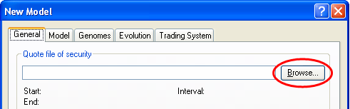
The “Model Configuration” dialog box will open, showing the “General” tab. The first thing to do is to select the quote file of the security that we are going to model. In this case we will use the included S&P500 index quote file.

At “Quote file of security”, click the “Browse…” button

In the “Browse” dialog box, open “S&P500 (Day).csv” (in the Samples folder)

The quote file will now be preprocessed to automatically detect the quote interval and some other settings. Note that the “Model evolution start date/time” is automatically set to a date shortly after the start of the quote file.

Near the bottom of the dialog box, check “Pause model after creation”

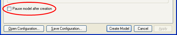
This will allow us to observe the model’s initial state before starting model evolution.

Select the “Model” tab

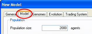
The “Model” tab contains various parameters. We will leave these at their default values. Notice that the population will contain 2000 agents. We will also leave the tabs “Genomes” and “Evolution” unchanged.

Select the “Trading System” tab

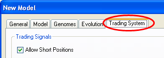
In the top-left you will see that “Allow short positions” is checked. This means that long, short and cash positions can be advised. In the “Trading Simulator” area, note that “Auto start at bar:” is checked with the value “2500”. This means that the built-in trading simulator will automatically start trading after 2500 quote bars have been processed. (The first 2500 bars can be considered a “training” period in this case). We will leave these settings as they are.

In the “Broker commission, spread and slippage” area we need to enter realistic transaction costs for the Trading Simulator. For SPY the spread is usually 1 cent which is about 0.01% of its value.

At “Average bid/ask spread %”, enter “0.01”

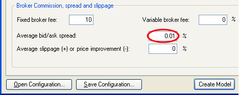
We will leave the other values unchanged. This concludes our model’s configuration.

Lesson 2: Model initialization

You are about to create and initialize the model:

Click the “Create Model” button of the “Model Configuration” dialog box

After clicking “Create Model” the model will be created and initialized. In this case, a population of 2000 agents is created and each agent is given a random trading rule, a starting capital of 100,000 in cash and no shares. (Shares in this case are fictitious “S&P500 index” shares). Model initialization takes only a short time and is only visualized by a progress bar.

When model initialization is complete, the following windows have appeared:

· Data Series: an expandable tree view with all of Adaptive Modeler’s data series (more about this later)

· Current Values: some values at the current point in model evolution (such as the number of bars that have been processed which is still zero now)

· Trading Signals: a list of recent trading signals (still empty now)

· Charts: several charts such as the S&P500 index price (most charts are still empty now)

This is the default “style” of Adaptive Modeler. A style is a workspace layout that includes various presentation settings and preferences. Now however, we are going to use another style that was specifically designed for this tutorial:

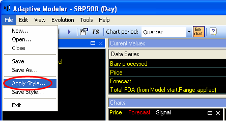
From the “File” menu, choose “Apply Style…”

In the “Open” dialog box, open “Tutorial.aps” (in the Styles folder)

The workspace has now been changed. The Charts window is now called “Model” and contains some other charts.

Tip: You can disable the Tool Tips that keep popping up when you move the mouse across the screen by going to the “Tools” menu, select “Options…” and uncheck “Show User Interface Tool Tips”.

Let’s take a brief look at the initial state of the model before starting model evolution.

As said, all agents own 100,000 in cash and 0 shares. This is visible in the “Wealth Distribution” histogram chart in the top-left of the Model window. This histogram is now showing a single bar representing 2000 agents that all have a wealth of 100,000.

Because all agents have 0 shares at this point, their “position” is 0%. This is shown in the “Position Distribution” histogram chart (top-center). The position of an agent is the value of the shares it owns as a percentage of its wealth. A negative value indicates a short position.

The top-right chart is a “Genome Size Distribution” histogram. Genomes are the trading rules of agents. The chart already shows that the trading rules have different sizes. The size is measured in the number of “genes” that the genome consists of. Genes are the elementary functions and values that trading rules are constructed of. The average genome size is shown in yellow on the X-axis. Later we will look at individual agents and trading rules in more detail.

Since you will be using this model throughout the rest of this tutorial, it is a good idea to save it now in case you need to revert to this point later.

Select “Save” from the “File” menu and save the model at a location of your choice

Now that we are familiar with the initial state of the model, we are ready to start model evolution.

Lesson 3: Model evolution

The model is ready to start its evolution. During evolution the model will process the historical quotes in the quote file as live streaming data. Every quote bar is processed only once and in chronological order. (Model evolution doesn’t end when the quote file ends or when present day is reached. It continues when new quotes are added to the quote file and there is no difference between the way historical and new quotes are being processed).

We will first go through model evolution step by step, feeding it one quote bar at a time:

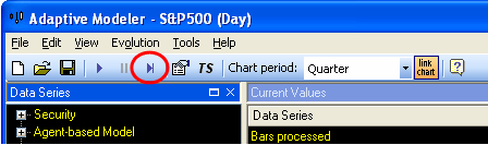
In the toolbar, click the “step” button (or press F4)

The model now evolves one step, starting at the “Model evolution start date/time” as set on the “General” tab of the model configuration (recall from Lesson 1). At every step, one quote bar is read from the quote file[12] and all agents evaluate their trading rule and place a buy or sell order on the Virtual Market. The Virtual Market (“VM”) calculates the clearing price and executes all executable orders. The clearing price (“VM Price”) is then taken as the forecast for the close of the next bar and a new trading signal is given if necessary. This process is repeated for every imported quote bar. A step usually takes only a fraction of a second.

Let’s see what exactly has changed after this first step. The first values have appeared in the charts “Buy Orders”, “Sell Orders”, “VM Trades”, “VM Volume” and “VM Price”. These reflect the numbers of buy and sell orders that have been placed, the resulting trades and the clearing price. More detailed market information such as market depth is also available but to keep things simple this is not covered in this tutorial.

The “Wealth Distribution” and “Position Distribution” histograms now show different wealth and position values for agents as a result of changes in their portfolios.

The forecast (which equals the VM Price) is shown in the Current Values window and also drawn in the bottom-right chart (in red). This chart also shows the security’s price in yellow (the S&P500 index in this case). A trading signal has been generated depending on whether the forecast is above or below the last security price and is shown in the Trading Signals window. The trading signal is also drawn in the bottom-right chart (in white) as an up or down arrow for “Long” or “Short” signals or a small circle for “Cash” signals[13].

Note: Depending on available space, the security price is shown in the chart as close lines or as OHLC bars.

Tip: You can maximize a chart or entire window to get a better view by clicking the “maximize” button near its top-right corner. Maximized charts or windows can be de-maximized with the “de-maximize” button. Depending on your screen size, you may want to maximize a chart or window at some points during this tutorial.

Press F4 (or click the “step” button) some more times while observing the charts

You will see the Virtual Market activity unfold further as new orders are placed by agents. The number of buy and sell orders and trades varies per bar. At every step a forecast for the next bar’s closing price is made. New trading signals will be given when necessary. Because Adaptive Modeler makes a bar-ahead forecast every bar (attempting to predict the direction of bar-to-bar price changes) new signals are sometimes given almost every bar.

Model evolution can also proceed continuously. Use the “resume” and “pause” buttons to resume/pause model evolution. You can also use the F3 key to resume/pause model evolution.

Press F3 a couple of times to resume and pause model evolution

We will now let the model evolve until about 1000 bars. You can see how many bars have been processed in the Current Values window. Use pause/resume (F3) or step (F4) at will. Take your time and observe the charts.

Evolve the model until about 1000 bars have been processed and then pause it again

Note: Especially during the early (“learning”) stages of model evolution, forecasts sometimes strongly diverge from the security price. Later the forecasts usually tend to stay closer to the security price. Therefore, the Trading Simulator is usually started after a learning period of a number of bars. Adaptive Modeler also offers ways to filter out strongly diverging forecasts (see Significant Forecast Range).

You may have noticed that after 80 bars the “Genome Size Distribution” also started to change. This is caused by the replacement of agents and their trading rules by new agents through breeding. We will talk more about this later.

Also note that the “Population Position” chart (bottom-center) shows the course of the average position of all agents over time.

Note: In case you failed to pause the model around 1000 bars and the model has already evolved much further, you can revert to the model saved at the end of Lesson 2 and try again in order to keep the model in sync with this tutorial. Saving the model at the end of every lesson is recommended for reverting when needed.

Controlling Charts

Because older information disappears from the left side of charts during evolution, the charts are now only showing the last quarter of history. This is indicated in the “Chart period” dropdown box in the main toolbar which shows “Quarter”. You can change the chart period to view longer periods:

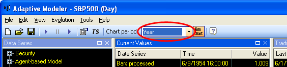
In the main toolbar, click on the “Chart period” dropdown box and select “Year”

All the charts (except the distribution histograms) will now show one year of history.

In “Chart period” dropdown box, select “5 years”

Now all the model’s evolution history so far should be visible.

In “Chart period” dropdown box, select “Quarter” again

To look back at older information without zooming out and losing details, you can simply scroll the charts horizontally:

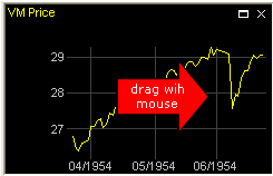
On the “VM Price” chart’s plot area, click and hold down the left mouse button and drag the chart to the right to see its history

When you do this, all the charts will scroll in sync (except the distribution histograms). When you are done viewing the history:

Drag the chart back to its most recent value again (or click the > button near the top-right corner to jump there directly)

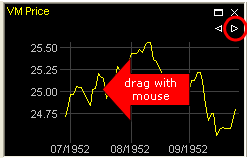
Note: A chart must be showing its most recent value in order to get automatically updated during model evolution. (When the most recent value is shown, the < and > buttons are not shown). To learn more about using charts, see Charts.

Lesson 4: Agents

In an agent-based model the most interesting phenomena are generally seen on the population level rather than in individual agents. The purpose of an agent-based model is to study emergent behavior caused by the interaction of many (relatively simple) agents. Likewise, we are more interested in the forecasts (Virtual Market prices) that result from our model than in the life and times of individual agents.

Nevertheless, it is important to know what agents are and how they operate and interact to understand how they influence their environment (the market) and the forecasts. In this lesson we will therefore first look at the details of individual agents before we look at the population as a whole again.

Viewing agent details

To get detailed information of an agent:

From the “View” menu, choose “Agent” and then “Agent 1”

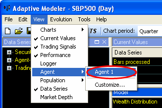
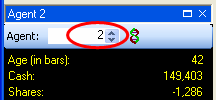
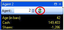
A window titled “Agent 1” has now appeared (bottom-left) showing the following information of agent number 1:

· Age: number of bars processed since agent creation

· Initial wealth: the agent’s wealth at the start of its creation

· Cash: amount of cash owned by agent

· Shares: number of shares owned by agent (negative for short position)

· Wealth: total wealth of an agent (value of cash and shares)

· Position: value of shares as a percentage of wealth (negative for short position)

· Cumulative (excess) return: return since agent creation (excess of security’s return)

· Breeding fitness (excess) return: a short term trailing (excess) return measure (selection criterion for breeding)

· Replacement fitness (excess) return: average (excess) return per bar since agent creation (selection criterion for replacement)

· Transactions: number of transactions an agent has done during its lifetime

· Trade duration: average number of bars between transactions (indicator of an agent’s investment/trading horizon)

· Volatility: volatility of agent wealth (indicator of absolute risk of an agent’s investment/trading style)

· Beta: correlation of agent wealth with security price (indicator of relative risk of an agent’s investment/trading style)

· Generation: genealogical generation number of agent

· Offspring agents: number of offspring agents that this agent has produced

· Genome size: size of genome (trading rule) in number of genes

· Genome depth: number of hierarchical levels in genome

Evolve the model until about 1300 bars (use F3 and/or F4) and watch the agent values change

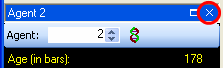
You may notice that Age is sometimes reset to 1. This means that the agent has been replaced by a new agent in the breeding process. In fact, the Agent window shows “slots” in the population. Also note that some agent values only become available when the agent has reached a certain age.

Look at some other agents by changing the agent (slot) number in the Agent window’s toolbar (by typing or by using the up and down buttons or keys)

Agent charts

Most agent values can also be followed in charts:

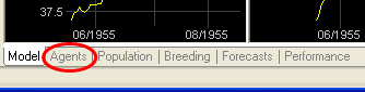
Click on the “Agents” tab (below the charts)

In this window, a chart with the wealth history of agent 1 is already showing. We will add some more charts:

In the Data Series window on the left, expand the “Agent-based Model” category

Expand the “Agent” subcategory

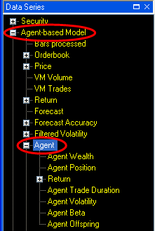
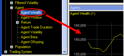
In the “Agent” subcategory you will see various agent data series such as “Agent Wealth” and “Agent Position”. To watch the trading activity of an agent:

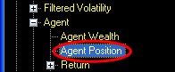
In the Data Series window, double-click on the “Agent Position” data series name

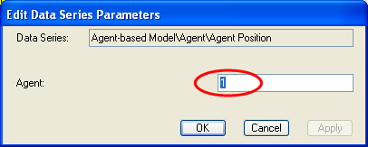
A dialog box “Edit Data Series Parameters” will appear where you can enter the agent number to show:

Enter “1” in the text box and press ENTER (or click “OK”)

A new chart showing the position history of agent 1 has now been added to the Agents window. It doesn’t contain any history yet because this information is not stored for all agents. During model evolution new information will appear in this chart. With this chart it is easy to see the transactions of an agent from the changes in its position.

You can also show information of multiple agents in one chart:

From the Data Series window, drag and drop the “Agent Wealth” data series name into the chart “Agent Wealth (1)”

Enter “2” in the “Edit Data Series Parameters” and press ENTER

The wealth of agent 1 and agent 2 is now shown together in one chart.

From the Data Series window, drag and drop “Agent Position” into the “Agent Position (1)” chart, enter “2” in the dialog box and press ENTER

The position history of agent 1 and agent 2 are now shown together in one chart.

Evolve the model until about 2000 bars and watch the agent charts

You may notice dots appearing in the agent charts occasionally. This indicates agent replacement.

Tip: You can show any data series from the Data Series window in a chart in the ways shown above. Up to eight data series can be combined in one chart.

Trading rules

From the Agent window, you can also view an agent’s trading rule.

In the Agent window’s toolbar, click the “Show genome” button

A window will appear showing the agent’s trading rule. Explaining the trading rules is outside the scope of this tutorial. To learn more, see Showing an agent’s genome or Trading Rules.

When you are done viewing the trading rule, close the trading rule window

Close the Agent window by clicking the x button in its top-right corner

Viewing the population

You are already familiar with the wealth and position distribution histogram charts. These charts give only a glimpse of the diversity of agents. A more extensive visualization of the agent population is provided by the Population window where multiple agent values can be plotted against each other.

Click on the “Population” tab (below the charts)

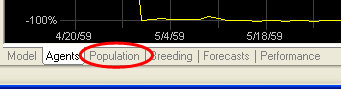
The Population window is now showing and contains a scatter plot of agent Wealth against agent Age. As is shown in the toolbar, Age is shown on the X-axis and Wealth on the Y-axis. Every dot represents one agent.

In the Population window’s toolbar, click the “Show Correlation and Regression” button

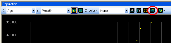
Correlation and regression information will appear and a regression line is drawn. In general, there will be a positive correlation between Age and Wealth because evolutionary selection pressure will let successful agents stay in the population longer than unsuccessful ones.

In the Population window’s toolbar, click on the “Z (color):” dropdown box and select “Position”

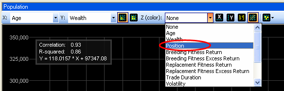
The color of the agents now indicates their position; blue for long positions and red for short positions (see the legend above the plot area). During model evolution you will notice agents changing color. Some agents are holding a long position most of the time, others a short position and others frequently switch positions.

Evolve the model until about 2500 bars while watching the Population window

Let’s look at some other agent values:

In the Population window’s toolbar, click on the “X:” dropdown box and select “Trade Duration”

Trade Duration is the average number of bars between successive transactions of an agent.

Click the “Show Correlation and Regression” button again to remove correlation and regression information

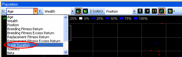
Agent Wealth is now plotted against Trade Duration. Agents with low trade duration (“active traders”) are on the left and those with high trade duration (“long term investors”) are on the right.

Evolve the model until about 3000 bars and watch the Population window

You may notice that some agents are moving to the right as their trade duration increases over time (“long term investors”) and others are staying on the left while frequently changing their Position as is visualized by color changes (“active traders”).

Hundreds of different scatter plots can be made from all the possible combinations of agent values. A quick way to see some of them is to browse through the “X:”, “Y:” or “Z:” dropdown boxes. To ensure that the most relevant region of the plot is automatically shown for every combination, the axes ranges can automatically be set to a number of standard deviations around the mean value:

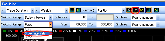
In the Population window’s toolbar, click the “X-Axis settings” button

In the X-axis toolbar that has just appeared, click on the “Range:” dropdown box and select “stdev intervals”

In the Population window’s toolbar, click the “Y-Axis settings” button

In the Y-axis toolbar, click on the “Range:” dropdown box and select “stdev intervals” as well

In the Population window’s toolbar, click the “X-Axis settings” and “Y-Axis settings” buttons once more to hide the axis toolbars

Now double-click on any of the “X:”, “Y:” or “Z:” dropdown boxes and use the mouse wheel (or UP and DOWN arrow keys) to browse through different plots

Evolve the model until about 6000 bars while browsing through different plots at will

Tip: An interesting plot is “Offspring” for X, “Genome size” for Y and “Beta” for Z. The horizontal position of agents now indicates the total number of their offspring agents (which in general correlates strongly with long term return). When an agent moves to the right, it is creating offspring agents and must therefore be among the agents with highest Breeding Fitness Return (which is a short term return indicator). The Genome size itself is not of major interest here but is used to distribute agents vertically over the chart for clarity. Because the genome size doesn’t change during an agent’s life, the vertical position stays fixed which makes it easy to follow individual agents.

Breeding

Breeding is the process of creating new offspring agents from some of the best performing agents to replace some of the worst performing agents. At every bar, agents with the highest “Breeding Fitness Return” are selected as parents. Copies of the genomes (trading rules) of pairs of these parents are then recombined through genetic crossover to create new genomes that are given to new offspring agents. These new agents replace agents with the lowest “Replacement Fitness Return”.

The breeding frequency and the number of agents to be replaced can be controlled by parameters to influence the adaptability versus the stability of the model. Changing these parameters is outside the scope of this tutorial but we will look at how some of the consequences of the breeding process can be observed.

Click on the “Breeding” tab (below the Population window)

In the main toolbar, set the “Chart period” to “25 Years”

The “Creations” chart (top-left) shows the number of agents created per bar. After some heavy initial fluctuations this value stabilizes to 20 agents per bar (1% of the population). (The initial fluctuations are because the number of agents that can be created/replaced depends on agent age). To keep the population size fixed, the number of replaced agents is always equal to the number of new created agents.

The “Avg Agent Age” chart shows the average age of all agents. This gives an indication of the level of experience present in the population. Sudden drops may indicate a sudden change in the market that resulted in a wipe-out of experienced agents. The “Age distribution” histogram shows what age groups currently exist in the population.

The “Avg Genome Size” shows the average size of the genomes over time. Also recall the Genome Size Distribution histogram on the Model tab. Through the process of recombining and mutating genomes for the creation of new agents, the average genome size changes. Bigger genomes may contain more complex algorithms and may be able to look back further in history but do not always necessarily perform better.

Evolve the model until the end of the quote file while observing the Model, Agents, Population or Breeding window at will (at any Chart period)

Lesson 5: Evaluating forecasting abilities

So far we have looked inside the model extensively but we have not looked at how well it is doing what it is supposed to do, forecasting prices. To evaluate the forecasting abilities of a model, a number of indicators are available.

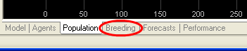
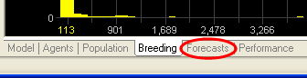
Click on the “Forecasts” tab (below the main window)

In the main toolbar, set the “Chart period” to “Quarter”

A simple but intuitive way to observe past forecasts is provided by the “Right Forecasted Price Changes” (blue) and “Wrong Forecasted Price Changes” (red) in the top-center chart. These series show the security price using blue for price changes whose direction was forecasted right and red for those that were forecasted wrong. This visualizes how many price changes were forecasted right and wrong as well as their magnitude.

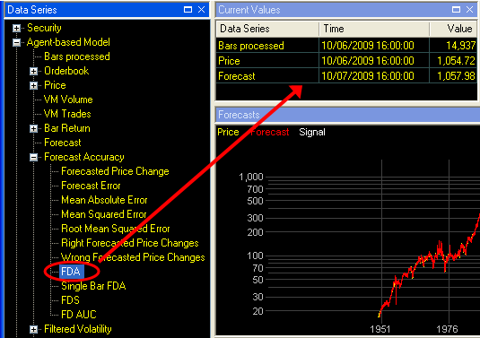
A more quantitative way to evaluate forecasts is provided by the “FDA” chart (top-right). FDA stands for “Forecast Directional Accuracy”. This indicator shows the percentage of bars for which the forecasted bar-to-bar price change was in the right direction. Values above 50% indicate that more often than not the direction of price change was forecasted correctly. The chart shows a 100 day trailing FDA during the last quarter.

To see how the FDA evolved during the entire model history:

In the main toolbar, set the “Chart period” to “100 Years”

On such long time scales you may want to calculate a trailing FDA over more bars:

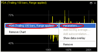
Right-click on the “FDA” chart

In the context menu, open the data series submenu and click “Parameters…”

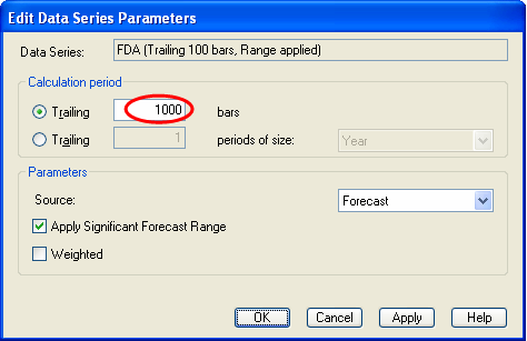
In the dialog box, enter “1000” at “Trailing … bars” and click “OK”

The chart now shows a 1000 day trailing FDA. You may notice that FDA varies over time. To get the average FDA over the entire model history:

In the Data Series window, expand the “Agent-based Model” category and expand the “Forecast Accuracy” subcategory

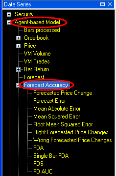
In the “Forecast Accuracy” subcategory, locate the “FDA” data series and drag and drop it into the Current Values window

In the “Edit Data Series Parameters” dialog box, select “Since model start” and click “OK”

The FDA since model start is now shown in the Current Values window.

Tip: You can drag any data series from the Data Series window into the Current Values window.

For a more complete evaluation of forecasting abilities, other indicators in the “Forecast Accuracy” subcategory of the Data Series window should be observed as well. This is outside the scope of this tutorial.

Tip: To learn more about any data series in the Data Series window, click on (or select) the data series name and press Shift-F1.

To conclude whether or not a model with forecasting abilities will be useful for trading, the performance of trading based on the trading signals needs to be evaluated. This performance does not only depend on forecast accuracy but also on volatility and transaction costs. In the next lesson we will see how to evaluate performance with the Trading Simulator.

Lesson 6: Trading Simulator

The Trading Simulator simulates trading based on the trading signals and the user’s trading preferences. It can be used to calculate returns and other performance indicators.

Click on the “Forecasts” tab and set the “Chart period” to “100 Years”

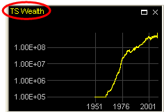
The “TS Wealth” chart (middle-left) shows the Trading Simulator Wealth[14]. To get its exact current value:

Click on the data series name (“TS Wealth”) above the chart

A data overlay will be shown on the chart with the value at the current bar.

Tip: You can get a data overlay for any data series in a chart by clicking on its name above the chart. Click once more to hide it again. To learn more see data overlay.

At model creation, Trading Simulator Wealth starts with the Start Capital as specified on the “Trading System” tab of the model configuration (100,000). While the Trading Simulator is enabled, it simulates trading according to the signals. Its wealth is adjusted accordingly, taking into account the broker commission, spread and slippage settings as specified on the “Trading System” tab. Recall from lesson 1 that the Trading Simulator was set to start trading automatically after 2500 bars (around 1960).

Tip: You can manually enable or disable the Trading Simulator during model evolution with the “TS” button on the main toolbar. You can also change Trading System settings and other model parameters during model evolution using the “Model Configuration” button on the main toolbar.

The middle-center chart shows a 1 year trailing return of the security (in yellow) together with a 1 year trailing return of the Trading Simulator (in red). The middle-right chart shows the excess 1 year trailing return of the Trading Simulator over the security[15].

The bottom-left chart shows the historical volatility of the security (in yellow) with the historical volatility of Trading Simulator wealth (in red). The volatility of Trading Simulator wealth is often somewhat lower than that of the security because the alternation of long, short and cash positions tends to temper volatility.

The bottom-center and bottom-right charts show the Trading Simulator position and its number of transactions per day[16]. On a period of 100 years these charts are not very clear. We will therefore add moving averages:

Right-click on the “TS Position” chart

In the context menu, open the submenu for the data series and click “Add moving average…”

In the “Edit Data Series Parameters” dialog box enter “1000” at “Bars” and click “OK”

A 1000 day moving average of the Trading Simulator position has now been added to the chart (in red).

In the same way, add a 1000 day moving average to the “TS Transactions” chart

Tip: You can add moving averages to most charts.

An overview of the Trading Simulator’s performance with various risk and return indicators is provided by the Performance Overview:

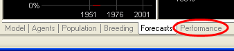
Click on the “Performance” tab (below the Model window)

The Performance Overview is now showing. You can change the calculation period and some other settings by clicking on the “Performance Calculation Settings” button at the top of the Performance Overview. To learn more, see Performance Overview.

Note: Model evolution, forecast accuracy and performance depend in part on random factors that are inherent to agent-based modeling and genetic programming. The model created in this tutorial will therefore be different every time it is created. In general it is recommended to do multiple runs using the same model configuration for a more complete overview of possible results.

Tip: For a more extensive analysis of the potential range of returns under varying conditions based on assumed values of FDA and volatility, the Statistical Simulations can be used.

Lesson 7: Creating your own models

This tutorial concludes with some guidelines for creating your own models. When creating your own models, a few things will usually be different than as shown in this tutorial.

Market data

Market data needs to be provided and may need to be converted to one of Adaptive Modeler’s supported formats. See 4. Market data for more information about this.

Model Configuration

At least the following model parameters should be checked/adjusted to correspond with the security that you are modeling and with your preferences (more about model configuration is explained in 5. Model configuration):

On the “General” tab:

After selecting a quote file, the “Model evolution start date/time” will automatically be set at the earliest possible start time (a certain number of bars after the first quote in the quote file). It is possible to set the start date/time to a later date/time.
Verify that the “Market Trading Hours” match the actual trading hours of the security and correct them if necessary.

On the “Model” tab:

Under Rounding, make sure that the number of decimal digits and minimum price increment unit are correct.

In the “Gene Selection”:

Enable/disable the open, high, low, bid, ask genes depending on which data is included in the quote file and whether or not agents should be able to see it. (Note that bid and ask also apply to the Virtual Market).
Enable/disable volume related genes depending on whether or not volume data is included in the quote file and whether or not agents should be able to see it.
Enable/disable genes related to custom input variables depending on whether or not these are included in the quote file and whether or not agents should be able to see them.

On the “Trading System” tab:

Check or uncheck “Allow short positions” and other trading signal generation settings as desired.
Enter a Start Capital for the Trading Simulator.
Enter the correct broker commissions, spread and slippage values for the security.

Model evolution

By default, the “Pause model at start” option is disabled so model evolution starts immediately after initialization. Often you may want to evolve a model first until present day without interruptions and then analyze the results afterwards (also see Computation performance issues). However, if you want to observe model evolution “live” using the Population window (or other data that is not stored historically) you can use the pause, step and resume functions.

Style

The default style that Adaptive Modeler uses is not the same as the style that was used for this tutorial and does not contain the same charts. However, you can select any style to be the default style or even create your own default style. To learn more, see Styles.

3. How does Adaptive Modeler work?

Adaptive Modeler consists of two main parts: the Agent-based Model and the Trading System. In short, the Agent-based Model receives quotes and produces price forecasts and the Trading System decides when a new trading signal should be given based on the forecasts and the user’s trading preferences.

Adaptive Modeler Components

3.1 Agent-based Model

The Agent-based Model consists primarily of a population of agents and a Virtual Market where agents can trade the security. An agent is an autonomous entity representing a trader (or investor) with its own assets (cash and/or shares) and its own trading strategy.

After initialization, a new model starts evolving by executing its regular cycle for every received quote bar as shown below.

Agent-based Model cycle

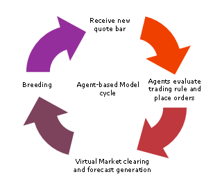
After a new quote bar has been received, agents can place a new order or remain inactive according to their trading strategy. After all agents have evaluated their trading strategy, the Virtual Market determines the clearing price, executes all executable orders and releases the price forecast for the next bar. Finally, breeding of new agents and replacement (by evolutionary operations such as crossover and mutation) can take place. This process then repeats itself for the next bar.

Note that in most cases (depending on model settings) the agent-based model is not a closed economy. The total amount of money in the model may vary because of agent replacements[17] and because of broker commissions charged to agents. New agents get an initial wealth (according to the Agent Initialization settings) that is usually different (higher) than the wealth of the replaced agents. On average this has an increasing effect on the total amount of money. When broker commissions are charged to agents these amounts are being discarded, which has a decreasing effect on the total amount of money. The total amount of money in the model can be observed with the Population Cash data series. Also the total number of shares that exist in the model can vary because of agent replacements. New agents get an initial shares position according to the Agent Initialization settings while the shares of the replaced agent are being discarded. The total number of shares in the model can be observed with the Population Shares data series.

3.1.1 Agent Population

At model initialization a population of agents is created according to the model parameters specified by the user. These parameters include the Population Size and the Agent initialization settings. The population size is generally thousands of agents. Upon creation, each agent receives a starting capital consisting of cash and/or shares depending on the distribution methods selected in the Agent initialization settings. Each agent also receives a trading rule (its “genome”) that is randomly created according to the Genome Settings.

After all initialization processes, the agent population will evaluate its trading rules, trade and breed according to the Agent-based Model cycle.

3.1.1.1 Trading rules

The trading rules use historical market data as input. This can be price or volume data of the security (either on the Real or Virtual Market) or custom input variables. According to their internal logic they return an “advice” consisting of a desired position (as a percentage of wealth) and an order limit price for buying or selling the security. A market order can also be indicated. The internal logic of the trading rules is built from several functions such as:

market data access functions
average, min, max functions on historical market data
logical and comparison operators
some basic Technical Indicators

The trading rules are created by genetic programming technology. Through evolution, the trading rules are driven to use those input data and functions that provide the most predictive value. For more information about how the trading rules are constructed, see III.2 Genetic programming in Adaptive Modeler.

3.1.1.2 Order generation

Adaptive Modeler translates the output of an agent’s trading rule (the “advice”) into a buy or sell order by comparing the desired position with the agent’s current position and calculating the number of shares that need to be bought or sold. If shares need to be bought or sold, an order will be generated to buy/sell the required number of shares, using the limit price or market order indication included in the advice.

Example:

An agent owns 1000 shares of the security and 80,000 in cash. The security’s price is 38,50. The agent’s wealth is therefore 118,500 and its position is 32.5%. If its trading rule returns an advice for a position of 50% and a limit price of 38,50, then a limit order will be generated to buy 539 (= 50% * 118,500 / 38,50 - 1000) additional shares for a limit price of 38,50.

Some implementation details:

The example given above is simplified. Actually, broker commission costs are included in the calculation as well.
Before translating an advice into an order, the desired position is limited to 100% of wealth for long position and -100% of wealth for short positions so that no positions are being entered that exceed these limits. Also an initial margin check is performed to verify that the agent’s new position (after the intended order would be executed) will still be within [-100%, 100%] of the agent’s new wealth, taking into account the difference between the order limit price and the last (Real Market) security price. If not, the number of shares to buy or sell will be reduced accordingly. (Note that an existing short position of an agent may later become less than -100% of wealth through an increase in the security price; also see Margin maintenance below).
If the difference between the desired position and the current position is less than half the Minimum position increment, no order is generated. This ensures that no order is being generated when the desired position is already equal to or close enough to the current position.
If an order does not get executed on the Virtual Market, the agent that placed the order will cancel the order before evaluating its trading rule again. If the new advice from the trading rule still requires a buy or sell order, an order will be placed again. This ensures that each agent can have only one order open at a time.
Depending on the Fractional shares setting, agents can trade fractional shares or only whole numbers of shares.
A long position can be changed into a short position and vice versa through a single transaction. In this case the fixed broker commission will be charged twice.

3.1.1.3 Margin maintenance

If the current position of an agent becomes less than -150% of its wealth (as a consequence of an increase in the security price), the agent will receive a “margin call”. This means that a buy order will be generated with a limit price set to 5% above the most recent price on the Virtual Market. (The desired position will be based on the current advice as normal since this is always at least -100%). Note that this mechanism does not guarantee that the short position will become higher than -150%. The number of margin calls occurring can be monitored with the Margin Calls data series.

3.1.1.4 Default management

If an agent's wealth becomes negative, it is forced to close any open position (regardless of available cash) by placing an order with a limit price 5% higher/lower than the most recent price on the Virtual Market. Once their position is closed, defaulted agents will be replaced in a special “defaults replacement” procedure by random created agents (if they weren't already replaced by the breeding operation). Note that defaulted agents may continue to exist as long as their position can not be fully closed and they are not being replaced by the breeding operation. It is theoretically possible that a defaulted agent (that has not yet been removed) recovers and gets positive wealth again. In that case it continues to exist as normal. The number of defaults occurring can be monitored with the Defaults data series.

3.1.2 Virtual Market

The Virtual Market is a simulated double auction batch market where all buy and sell orders from agents are collected. Every bar, after all agents have evaluated their trading rule and placed their order (if any), the Virtual Market calculates the clearing price. The clearing price is the price at which the highest trading volume from limit orders can be matched[18]. The Market Depth window shows the depth of the orderbook before and after clearing. There is no market maker. When the total number of shares offered (at or below clearing price) exceeds the total number of shares asked (at or above clearing price) or vice versa, the remaining orders will not be (fully) executed. In this case, orders at the clearing price will be selected for execution with priority for market orders over limit orders and then on a first‑in‑first‑out (FIFO) basis. Orders can be partially executed. In case there are no matching limit orders at all, no market orders will be executed either.

The forecast for the real market price can be based either on the clearing price of the Virtual Market (Virtual Market Price) or on only the buy and sell orders of a dynamically changing group of the best performing agents (Best Agents Price). In the default configuration the Virtual Market Price is used. The rationale for using the Virtual Market Price as an indicator for future prices is as follows: Because of the volume weighted clearing price computation mechanism, wealthier (more successful) agents (who will generally place bigger orders) will have a bigger influence on the market price than less wealthy (less successful) agents. This way the forecast calculation mechanism has a preference for successful trading strategies but still includes a high number of diverse trading strategies. The latter is needed to make the forecasting mechanism more robust to changes in market behavior since previously successful trading strategies are not guaranteed to remain successful in the future.

In some cases, using the Best Agents Price as the forecast may result in better forecasts. Other than that, it may be interesting to compare the forecasting abilities of the entire Virtual Market with those of a (much smaller) group of only the best performing agents.

3.1.3 Breeding

Breeding is the process of creating new agents to replace poor performing agents. Breeding occurs by selecting pairs of well performing agents (parents) and producing new genomes by recombination of the parent genomes through a crossover operation. In a crossover operation, the parent genomes are copied and then a randomly chosen part of the copied genome of one parent gets exchanged for a randomly chosen part of the copied genome of the other parent. The resulting two new genomes are used to create two new agents. Breeding can occur every bar or every n bars where n is the breeding cycle length.

3.1.3.1 Selection of parents

Parents are selected according to the parameters Minimum breeding age, Eligible selection, Parents group and Parent selection method. First the eligible selection is made. This is a temporary sub population in which breeding and replacement will take place. The eligible selection consists of agents of minimum breeding age or older, either all of them or a random selection of specified size. Then the best performing agents (judged by Breeding Fitness Return) of the eligible selection are selected as parents using the specified Parent selection method. The number of parents selected is specified by the Parents group size parameter. For more information about the selection process, see the parameter descriptions.

3.1.3.2 Creating offspring

The selected parents are randomly grouped in pairs. For each pair the crossover operator picks a random node in a copy of one parent’s genome and then selects another random node (of the same type) in a copy of the other parent’s genome. The subtrees starting at the selected nodes are then swapped.

To be accepted, the resulting offspring genomes must meet the Maximum Genome Size and Maximum Genome Depth constraints and must be different than their parent genomes. The crossover operator will attempt to exchange subtrees that are big enough to meet the specified Preferred minimum number of nodes. If Create unique genomes is checked, the offspring genomes must also be unique within the current group of parents and offspring. If not accepted, the crossover is retried until acceptable offspring genomes have been created or a time limit is exceeded. (In some cases crossover may not be possible, resulting in less offspring agents being created).

The resulting offspring genomes may then be mutated, according to the probability given in the Mutation probability parameter. Finally, two new agents are created and provided with the offspring genomes and a starting capital consisting of cash and/or shares according to the distribution methods selected in the Agent initialization settings.

3.1.3.3 Replacing agents

The created offspring agents will replace the worst performing agents of the eligible selection (judged by Replacement Fitness Return). Note that the number of agents that are being replaced is always equal to the number of offspring agents that have been created. This is to keep the population size stable.

3.1.4 Model Evolution

In the early stage of model evolution the forecast may sometimes diverge strongly from the security’s price. In this case the Virtual Market is acting chaotic because of an imbalance in supply and demand. This imbalance is caused by the fact that at model start the initial position of agents may not be in line with their trading rules. Therefore the agents first need to align their portfolio with the advice from their trading rule which can cause heavy trading volumes and big price changes.

As the model evolves two things will happen: First, agents that happen to have a well performing trading rule will become wealthier than less fortunate agents. Because they are wealthier they will have more influence on the Virtual Market price (the forecast) which presumably is beneficial to the accuracy of the forecast. Second, the trading rules will improve by natural selection as breeding creates new trading rules from the best performing rules, replacing the worst performing rules. For the purpose of selecting agents for breeding, the agent fitness is determined by the Breeding fitness return data series. For the purpose of selecting agents to be replaced, the agent fitness is determined by the Replacement fitness return data series.

The Agent-based Model is in fact a self-organizing system that evolves according to a balanced interplay of two mechanisms:

evolution of trading rules by genetic programming (micro level)
co-evolution of agents through trading on the Virtual Market and the resulting price dynamics (macro level)

3.1.4.1 Running multiple model evolutions

The evolution and results of multiple models that were all based on the same historical quotes and the same model configuration can be different. This is caused by the use of random numbers which is inherent to agent-based modeling and genetic programming. Random numbers are for instance used for the creation of trading rules. Only when the same random seed values are used, multiple models will evolve in exactly the same way[19].

This means that for a given security and a given set of parameter values, it may be necessary to do a number of runs to get a more reliable and complete overview of possible results. See also Batch processing and automation.

3.2 Trading System

The Trading System consists of the following components:

Trading Signal Generator
Trading Simulator
Statistical Simulations

3.2.1 Trading Signal Generator

After every generated forecast (every bar), the Trading Signal Generator evaluates whether or not a signal should be generated. Trading signals are generated based on the following factors:

forecast
last security price (on which the forecast was based)
“Allow short positions” parameter
“Significant Forecast Range” parameters
“Generate Cash signal when forecast is outside range” parameter
“Generate Cash signal at market close” parameter (only for intraday models)
“Apply FDA filter” parameter and corresponding FDA filter settings

In general, when the forecast is higher (lower) than the last price (and the absolute difference is within the Significant Forecast Range) then a Long (Short) signal will be generated. However, if “Allow short positions” is disabled, a Cash signal will be generated instead of a Short signal.

If the forecast is equal to the last price (or the difference is outside the Significant Forecast Range) and “Generate Cash signal when forecast is outside range” is selected, then a Cash signal will be generated. If the latter is not the case, then no new signal will be generated.

For intraday models, when “Generate Cash signal at market close” is enabled, a Cash signal will be generated every time the market closes, to avoid overnight positions.

A signal will only be generated when the new suggested position differs from the last generated signal. Therefore, signals remain valid until a new signal is given.

3.2.2 Trading Simulator

The Trading Simulator simulates trading according to the trading signals and the relevant Trading System parameters such as Start Capital, Broker Commission, Spread and Slippage (see 5.5 Trading System parameters).

When the Trading Simulator is enabled, it enters a long position in the security when a Long signal has been generated (with 100% of total capital and after closing any short position) and enters a short position when a Short signal has been generated (for 100% of total capital and after closing any long position). If a Cash signal has been generated then the Trading Simulator will hold only cash (after closing any position). When Trading is disabled, the Trading Simulator will not trade (any open position will be closed first). When the Trading Simulator gets enabled, it will first open a position based on the last generated signal.

For more information on using the Trading Simulator, see 7.2 Using the Trading Simulator. For more information on viewing its performance see 6.7 Performance Overview. Note that all return and performance indicators in Adaptive Modeler are calculated after all costs (broker commissions, spread and slippage).

3.2.3 Statistical Simulations

While the Trading Simulator shows the past and present trading performance of a particular model, it does not give insight into the potential range of (future) trading returns of multiple models (runs) and its sensitivity to various factors.

The Statistical Simulations included in Adaptive Modeler estimate the likely range of returns given various underlying factors. The simulation tools included are Historical Simulation (HS) and Monte Carlo Simulation (MCS). Both are implemented as data series and are further described in 7.3 Statistical Simulations and I.3.3 Statistical Simulations.

It is important to understand that the Statistical Simulations do not use any output from the Agent-Based Model (such as forecasts or trading signals). Instead they are based on user given expectations of Forecast Directional Accuracy and Forecast Directional Significance and on the return distribution of historical security prices (HS) or user given expectations of drift and volatility (MCS). Also they are affected by certain Trading System parameters and (optionally) the current Trading Simulator wealth.

4. Market Data

Adaptive Modeler needs an amount of historical market data that provides a sufficient learning period for model evolution. This is also needed for a statistically significant assessment of forecasting performance during different market trends. In general, at least 1,000 bars of historical data is recommended. Adaptive Modeler can process both OHLC bars as well as tick data. Bid and Ask prices and Volume data can also be used, as well as values of additional custom input variables[20]. In some cases historical data may need to be preprocessed by the user for best results (i.e. back-adjusting of futures contracts).

4.1 Data retrieval

Adaptive Modeler reads quotes from Comma Separated Values (CSV) files in familiar formats such as those used by popular charting and technical analysis software packages. Most data vendors and quote downloaders support exporting quotes to CSV files. Also various third party conversion tools exist. For example, the following data feeds can be exported to CSV files in real-time with an additional tool:

eSignal (with QCollector Expert)
DTN IQFeed (with QCollector for DTN IQFeed)

4.1.1 Required quote data

As a minimum, the following columns are required in the quote file:

Date
Close

Note that for tick data the Close column should be used for trade prices.

4.1.2 Optional quote data

The following columns are optional and can be used by Adaptive Modeler:

Time
Open
High
Low
Volume
Bid
Ask
Custom… (for custom input variables)

Other columns may also be included in quote files (usually this requires a header) but will be ignored by Adaptive Modeler.

Note: if Open, High and/or Low values are not included in the quote file, the following values will be assigned to them: Open will be set equal to Close, High will be set equal to the highest of Close and Open, and Low will be set equal to the lowest of Close and Open. If Open, High, Low or other values should not be visible to agents, then the corresponding genes should be disabled in the Gene Selection.

4.1.3 Accepted quote intervals

Adaptive Modeler supports any quote interval ranging from 1 millisecond to multiple days provided that processing time per quote is short enough[21]. For high-frequency data, the actual usable minimum interval thus depends on situation specific factors such as CPU speed, model parameters and data retrieval latency. Usually, processing time per quote is only a fraction of a second.

The quote interval size is automatically detected from the quote file. Variable intervals (i.e. for constant range bars or tick data) are also supported. If a variable interval is detected, an average (rounded) interval size is calculated for practical purposes such as charting[22].

4.1.4 Quote bar timing convention

The time field of a bar in the quote file should indicate the bar’s closing time. For this reason, the quote file should not contain bars with the market’s opening time. For End‑of‑Day files without time field, Adaptive Modeler will assign the market closing time (as set in the model configuration) to every bar.

4.1.5 Splits and dividends

Adaptive Modeler does not automatically adjust for splits and dividends.

As stock splits have a distorting effect on model evolution and on return calculations, the quote history file should be adjusted for splits before creating a model. When a new split occurs, a new model should be created after re-adjusting the historical quotes.

Whether or not historical quotes should be adjusted for dividends and by which method depends on situation specific factors and should be considered by the user. Note that return calculations in Adaptive Modeler do not include dividend payments.

Note that it may be necessary to change the rounding settings when historical prices have become very low after adjusting for splits and/or dividends.

4.1.6 Missing or irregular quotes

If a quote is found with a time other than the expected time, a notification will appear in the Log (see 6.10 Log). For example, quotes could be missing because of holidays, incomplete data or other reasons or quotes could be outside the regular Market Trading Hours. Missing or irregular quotes are not necessarily a problem (i.e. they could simply indicate a holiday) so normal operation will continue. However, they are being reported to the Log so that the user can see them. By viewing the Log, you can instantly check for missing quotes or other irregularities. For variable intervals, only notifications about quotes outside the Market Trading Hours will be reported.

4.1.7 Decimal digits

The number of decimal digits that imported quotes are rounded to can be specified by a model parameter (see Decimal places). This applies to Open, High, Low, Close, Bid and Ask values. After selecting a quote file in the “Model Configuration” dialog box, Adaptive Modeler will attempt to automatically detect the number of decimal digits that are used in the quote file and set the rounding parameter. You should check this value and adjust it if necessary.

4.1.8 Custom input variables

It is possible to include data from one or more custom input variables of choice in the quote file[23]. A custom input variable can be any variable that may be helpful for forecasting the security such as fundamental data (i.e. earnings, book value), economic indicators (i.e. GDP growth, jobless claims, industrial production, consumer sentiment), other price series, indices, bond yields, or a custom technical indicator calculated on the security price.

Custom input variables must be placed in extra columns named “Custom…” where “…” can be anything. If more than one custom input variable is used, they should all have different names. For example, three custom variables could be named “Custom1”, “Custom2” and “Custom3”, or “Custom_IBM”, “Custom_AAPL” and “Custom_MSFT”.

A maximum of 100 custom input variables is supported. In general, it is recommended to keep the number of custom input variables low, as it will be difficult for the system to discover the most predictive input variables among many (noisy) other ones. When using many custom input variables, a larger population size will increase the chance of the most predictive variable(s) being found.

Custom input variables may have negative and zero values. The values are not rounded on importing. When the value of a custom input variable is not specified for a bar (empty field), the last specified value will be used. Therefore it is not necessary to repeat the same value for several bars if the variable only changes periodically[24].

For agents to be able to make use of custom input variables, at least the following genes must be enabled in the Gene Selection:

· one or more of the genes custom, avgcustom, mincustom, maxcustom

· the >_custom gene and/or the change_cu gene

· one or more of the Digit genes (see Digit0, …, Digit9 and custom for how this works)

4.1.9 Quote reading process

As a model evolves, it will process all quotes in the quote file. When all quotes have been processed, the system will continue to read and process new quotes as soon as they are added to the quote file. There is in fact no difference between the way the system goes through historical quotes and the way it processes new quotes, except that the latter will go slower as it involves waiting for every new quote. (Note that the Evaluation Edition processes recent quotes only after a delay of a few days).

4.2 Quote file format requirements

Most quote files that use common formats will automatically be read correctly by Adaptive Modeler without conversion. When only using Open, High, Low, Close and Volume data, a header is usually not necessary. Several date and time formats are automatically recognized. It is also possible to use a header row to specify the columns and the date and time formats to override automatic detection.

4.2.1 Quote files without header

In many cases a header is not necessary. If no header is included then only Date, Time, Open, High, Low, Close, Volume and Open Interest columns are allowed and they must be in this order (only Date and Close are required). Open, High and Low columns may only be included all or none. Open Interest may only be included if Volume is also included (but will be ignored).

The date format will automatically be detected. If a Time column is included, the time must use a colon to separate hours, minutes and seconds. It is also possible to combine the date and time in one column, separated by a space.

Some examples of valid quote rows when not using a header (headers shown here only for clarification):

Date, Close

04/29/2009,64.75

Date, Time, Close

04/29/2009,10:15,64.75

Date, Time, Open, High, Low, Close

04/29/2009,10:15,64.25,65.00,64.00,64.75

Date, Time, Open, High, Low, Close, Volume

04/29/2009,10:15,64.25,65.00,64.00,64.75,548000

Date, Open, High, Low, Close, Volume, Open Interest

05/22/2009,244.00,251.00,243.50,249.50,1380,6858

4.2.2 Quote files with header

With a header, more possibilities are supported. Bid and Ask prices can be included and also custom input variables. Other columns may also be included in the quote file but will be ignored. Columns may be in any order and Open, High and Low columns may be included or excluded in any combination. The date and time format can (optionally) be specified exactly in the header to override automatic detection and avoid any ambiguities. Also time formats without colons are supported such as “hhmm”.

Some examples of valid quote rows when using a header:

Date,Time,Open,Close

29-Apr-2009,1015,64.25,64.75

Date,Time,Bid,Ask,Close,Volume,Custom1

04/29/2009,10:29:56.201,41.04,41.05,41.05,200,0.59

DDMMYYYY,Time,Open,High,Low,Close,Vol,Custom_IBM,Custom_AAPL

03042009,11:25,61.20,61.40,61.15,61.35,2200,102.22,115.99

$IBM,20090429,101.98,105.00,101.67,104.04,9783700

"Date","Open","High","Low","Close","Volume","OI"

05/22/2009,244.00,251.00,243.50,249.50,1380,6858

4.2.3 Supported date formats

All common date formats are supported. Some examples of supported date formats (not exhaustive):

Date format	Example date
yyyy-mm-dd	2009-04-29
mm/dd/yyyy	04/29/2009
dd.mm.yyyy	29.04.2009
dd-mmm-yyyy	29-Apr-2009
yyyymmdd	20090429
yy-mm-dd	090429

Many other variations are supported as well.

The date format usually does not need to be specified in a header and will be detected automatically. In some cases a large number of quotes may be needed to detect the month/day/year order in the date format unambiguously, especially for intraday files. In that case it may be necessary to use a header that contains the exact date format string. For example:

dd-mm-yy,Time,Bid,Ask,Close,Volume

03-02-03,9:34:21.873,35.73,35.74,35.73,100

The month/day/year order in the date format must stay consistent throughout the quote file.

In case the quote file contains quotes before 1/1/1930, four digits must be used for the year.

4.2.4 Supported time formats

All common time formats are supported. Some examples of supported time formats (not exhaustive):

Time format	Example time
HH:mm	15:45
HH:mm:ss.fff	15:45:23.863
h:mm:ss tt	3:45:23 PM
HH:mm:ss	15:45:23
HHmm	1545
HHmmss	154523

Several other formats are supported as well.

Hours may be in either 24-hour clock system or 12-hour clock system with AM/PM indication.

Fractional seconds can be specified in up to 3 decimal digits. Either a period, comma or colon may be used as the decimal separator.

If necessary the exact time format may be specified in a header.

Date and time may also be combined in one column, separated by a space[25].

4.2.5 Delimiters

The field (column) delimiter may be a comma, semicolon or tab.

4.2.6 Decimal separator

The decimal separator may be either a period or a comma (if not used as the delimiter).

4.2.7 Thousand separators

Price and volume values may contain thousand separators in the following ways: If a period is used as the decimal separator, then commas may be used as thousand separators but the value must be enclosed within double quotation marks. If a comma is used as the decimal separator, then periods may be used as thousand separators.

4.2.8 Column headers

Column headers may be field names such as Date, Time, Open, High, Low, Close, Volume (or Vol), Bid, Ask, or custom input variable names (“Custom…”).

For the date and time columns, also date and time format strings are allowed to specify the exact date or time format. When the date and time is combined in one column, this can be indicated by DateTime or a combined date/time format string to specify the exact format (i.e. “M/d/yy HH:mm:ss”).

Field names are not case-sensitive. Field names may also be included within “<” and “>” or within double quotation marks. Unknown field names will cause the data in that column to be ignored.

4.2.9 Interpretation of empty fields

Empty rows or rows containing only empty fields will be skipped. Empty fields are formed by adjacent commas, commas at the start or end of a line or fields containing only white space. Empty fields are processed as follows: Empty Date, Time or Close fields will result in an error message. Empty Open fields will result in the Close value being assigned to them. Empty High or Low fields will result in the Open or Close value assigned to them depending on which is higher/lower. Empty Volume fields will result in a 0 volume value. Empty Bid or Ask fields will result in a 0 bid or ask price[26]. Empty custom input variable fields will result in the most recent specified value being assigned to them.

Note that empty fields (extra commas) at the end of a line are sometimes not visible in spreadsheets such as Microsoft Excel. Therefore it can be helpful to inspect the quote file in a text editor in case of problems.

4.2.10 Miscellaneous requirements

Quotes must be in ascending order of date/time.
All lines must end with Carriage Return (0x0D) and Line Feed (0x0A) characters (CR+LF).
Close prices must be positive (not zero or negative).
Quote files should contain at least 250 quotes.
Intraday quote files should span at least a 24 hour period or contain at least 500 quotes.
If a quote file is renamed, moved or deleted during the lifetime of a model that uses it, the model will ask for the new location of the quote file when it needs it again. The new quote file should contain the same columns as the old quote file and the month/day/year order in the date format should still be the same as before.
If historical quotes in a quote file that is being read by Adaptive Modeler are being modified, the original quotes may have already been read into a buffer (while the current model date is still before those quotes) and the modifications may not be read anymore. The buffer size is about 100 lines so quotes within 100 bars from the current model date should not be modified anymore.

5. Model configuration

When creating a new model[27], various model parameters can be configured in the “Model Configuration” dialog box. Most parameters can also be changed during model evolution by selecting “Model Configuration…” from the “Edit” menu. Note that while editing parameters during model evolution, the model continues to evolve in the background (if not paused) using the original parameter values. Parameter changes will only become effective after clicking “OK” or “Apply”.

The various tabs and fields of the “Model Configuration” dialog boxes are discussed in this chapter.

5.1 General parameters

The following parameters can be found on the “General” tab:

5.1.1 Quote history file of security

Here the quote file of the security can be selected. This must be a valid quote file as described in 4. Market data. The quote file will be preprocessed to determine the quote interval and Market Trading Hours and to do some other checks. After preprocessing the quote file, the date and time of the first and last quote and the quote interval will be shown.

5.1.2 Security name/description

This will automatically be set to the name of the quote file but you can change this to any desired name or description.

5.1.3 Model name

After selecting a quote file, the model name is automatically set to the name of the quote file. You can change this to something else. The model name will be used as the default filename when the model is being saved for the first time. After the model has been created, the model name can only be changed using the “SaveAs…” command from the “File” menu.

5.1.4 Model evolution start date and time

The model’s evolution start date and time will automatically be set to the earliest possible start date and time. This is a certain number of bars after the first quote in the quote file. This is because the trading rules need some historical quotes before the model evolution start date. It is possible to set the start date and time to a later date and time. The start date needs to be entered in the format shown to the right of the input field. (This is either the US or European date format and depends on the date format selected in the “Options” dialog box).

5.1.5 Market Trading Hours

The Market Trading Hours represent the open and close times of the real world market where the security is being traded. They are used to calculate the amount of daily trading time which is used for accurately calculating compound return or volatility data series per compounding interval. Also they are used to calculate the expected date/time of the next bar that is being shown (temporarily) in the Current Values window and in charts[28].

The Market Trading Hours settings do not affect model evolution, nor forecasts and signals. Also they do not affect when new quotes are being processed, nor when forecasts and signals are being generated. This is because new quotes are being processed as soon as they appear in the quote file which is followed immediately by the generation of a new forecast.

Note that regardless of the Market Trading Hours settings, all quotes in the quote file will be used. If Pre‑Market or After‑Hours quotes should not be used then they should not be included in the quote file.

When a quote file has been selected, the Market Trading Hours are automatically determined using the times of the earliest and latest bars during the first few days of the quote file. You should verify that the Market Trading Hours are correct because it may not always be possible to derive the correct hours from the quote file. Especially the following cases may require attention:

· Intraday quotes from continuous 24h markets (i.e. forex)
In this case the opening and closing times will both automatically be set to 0:00h. Both times should manually be changed to the market closing time at the end of the week (using the same time zone as the times in the quote file). For continuous markets Adaptive Modeler assumes that the market will open again exactly 48 hours after the closing time on Friday.

· Non-integer number of quote intervals per day
If the number of quote intervals per day is not a whole number (i.e. hours on a market that opens at 9.30h and closes at 16.00h) and in the quote file the last bar of the day has a time later than the market closing time, then the market closing time should be set to the actual market closing time and not to the time given to the last bar (the bar will still be imported though).

· Quote intervals smaller than 1 minute
When the quote interval is smaller than 1 minute, the Market Trading Hours may not have been detected correctly and may need to be corrected manually.

· Variable quote intervals
When a variable interval is used, the Market Trading Hours may not have been detected correctly and may need to be corrected.

5.1.5.1 Handling changes in Market Trading Hours

While evolving a model, Adaptive Modeler can automatically check the quote file for changes in the security’s trading hours and adjust the Market Trading Hours. This is useful in case Pre‑Market or After‑Hours trading periods were added during the quote history or when expansions of these periods or of the regular trading hours occurred during the quote history[29]. There are three ways of dealing with adjustments:

1. automatic checking and adjustment

2. automatic checking, prompt for adjustment

3. no automatic checking or adjustment

The best way depends on whether changes can correctly be detected automatically (which in turn depends on the regularity of the quote file, missing bars, etc.) and whether or not you want model evolution to be interrupted for manual adjustments. In general it is recommended to check the Log for notifications such as “Missing Quote” or “Quote not within Market Trading Hours” to see if the Market Trading Hours are still correct and have been changed correctly during model evolution. These notifications occur occasionally which is normal but when there are many this could indicate that the Market Trading Hours are incorrect.

In any case you can still change the Market Trading Hours manually using the “Model Configuration” dialog box. This may be necessary for instance for overriding an automatic change, forcing an undetected change or for reducing Market Trading Hours.

Note that historical changes of the Market Trading Hours are being recorded and are used to calculate the number of actual periods (by market trading time) between bars for accurate calculation of returns, volatility and other indicators.

5.1.6 Pause model after creation

Check this to indicate that the model should be paused immediately after initialization of the agent population. This makes it possible to observe the initial state of a model before any quotes have been processed.

5.2 Agent-based Model parameters

These parameters refer to the Agent-based Model and can be found on the “Model” tab.

5.2.1 Population Size

The population size is the number of agents in the Agent-based Model. Bigger populations means that more different trading rules are competing and evolving in parallel at the same time. This increases the chance that profitable new trading rules emerge on time when new profit opportunities in the market arise. A bigger population also increases the ability of a model to endure different market regimes since more different strategies can be stored in the population. A larger population size also increases model stability and prevents models from becoming chaotic with extreme forecasts or from reaching a state of imbalance where no agent orders can be matched and no forecasts can be produced. Bigger populations also reduce sensitivity to random numbers so that results of different runs vary less. However, bigger populations require more computations and make model evolution slower.

Note: Very large models may take a while to save and open. A model of 250,000 agents can take about 30 seconds to save and 90 seconds to open. The model file size can get over a gigabyte. During saving/opening, the application may appear unresponsive.

5.2.2 Agent Initialization

By clicking the “Agent Initialization” button, a window will open with settings for the initialization of agent wealth and position (asset allocation). This concerns the start values of wealth and position that are assigned to new agents during model initialization and to new agents that are created through breeding during model evolution. Several methods are provided to assign initial wealth and position values to agents which will be described in detail below. Note that the resulting initial distributions can easily be observed by using the Pause model after creation setting and then showing the Wealth Distribution and Position Distribution data series in charts.

5.2.2.1 Wealth distribution

In general, it deserves mentioning that the initial wealth that is assigned to an agent has an impact on the amount of influence that the agent can have on the Virtual Market price because of the volume weighted pricing mechanism. When initial wealth is assigned to agents by any of the random sampling methods described below, this can add noise to the price discovery mechanism. To avoid such noise, assign equal initial wealth to all agents.

Initial wealth can be assigned to new agents by any of the following methods:

Equal for all agents

All agents get the same initial wealth. The amount can be specified at “Initial wealth”.

Pareto distribution

Agent wealth is randomly sampled from a Pareto distribution. The Pareto distribution is a well known power law distribution commonly used to describe wealth or income distributions. In particular it describes an unequal distribution where a large part of total wealth is owned by a small percentage of individuals (also known as the Pareto principle or “80-20 rule”). This distribution is generally considered to apply best to the distribution of wealth among very rich individuals and not necessarily to the rest of the population. A Pareto distribution has two parameters: the “Minimum wealth” and the “Pareto index”. The minimum wealth must be greater than zero. The Pareto index is a value greater than zero (usually between 1 and 3) that indicates the (un)evenness in income distribution. The higher the Pareto index, the more even the distribution is.

Maxwell-Boltzmann distribution

Agent wealth is randomly sampled from a Maxwell-Boltzmann distribution. This is an exponential distribution originating from the field of statistical mechanics for describing the distribution of energy of atoms in a gas. In econophysics, its general significance has been recognized for describing the distribution of a conserved quantity (such as money) among elements of a closed system (such as agents in an economy)[30] [31].

Note that although money may be considered conserved in a closed economy, wealth (when it includes non-cash assets) is not necessarily conserved. Wealth may change due to changes in asset prices or through the creation and destruction of assets[32]. Furthermore, a model in Adaptive Modeler is in most cases not a strictly “closed economy” (see here). However, for the purpose of assigning initial wealth values to agents, these inconsistencies are relatively minor, especially when the initial position (asset allocation) of agents is set to 0%.

The Maxwell-Boltzmann distribution has a parameter a which influences the magnitude of values (more precisely: a = rms²/ 3, with rms being the root mean square of the values).

5.2.2.2 Position distribution

In general, it should be noted that the initial position that is assigned to agents has a big impact on the total (net) number of shares that exist in the model and could therefore cause a bias or unbalance in the model, especially when it is strongly positive or negative. This could result in unstable models or lack of trading. To prevent this bias or unbalance, set the (average) initial position value to 0%. (Note however that the total number of shares that exist in the model also varies during model evolution because of agent replacement).

Furthermore, an agent’s initial position will usually be changed immediately after its creation as a consequence of trading according to its trading rule. The position distribution may therefore diverge from the chosen initial distribution during model evolution.

Initial positions can be assigned to new agents by any of the following methods:

Equal for all agents

All agents get the same initial position. The position can be specified at “Initial position” and must be within [-100%, 100%].

Uniform distribution

Agent position is randomly sampled from a uniform distribution within the specified range. So this means that all positions within the specified range have an equal chance of occuring. The minimum and maximum values must be within [-100%, 100%].

Gaussian distribution

Agent position is randomly sampled from a Gaussian (Normal) distribution with the specified mean and standard deviation. The mean must be within [-100%, 100%]. After random sampling, any position value less than -100% will be set to -100% and any value greater than 100% will be set to 100%.

5.2.3 Minimum position increment

This is the minimum increment (stepsize) of advised positions, as a percentage of wealth. This value is returned by the LevUnit gene. It can not be changed during model evolution. It is also used for checking whether an agent order would be of sufficient size to be actually placed (see Order generation).

5.2.4 Allow fractional shares

When this is checked, agents are allowed to buy and sell fractional numbers of shares. When this setting is unchecked, agents can only trade whole numbers of shares. Allowing fractional shares can be useful (and realistic) in case the security’s price is (gets) very high in relation to the wealth of (some) agents.

5.2.5 Broker commission (for agents)

These are the virtual costs per buy or sell transaction charged to agents for trading on the Virtual Market. By default the values for Broker Commission of the Trading System are used here but other values can also be provided. A fixed fee (amount) can be specified and/or a variable fee (percentage of transaction value).

5.2.6 Forecast

Here you can specify whether the forecast should be based on the Virtual Market Price (which is the clearing price on the Virtual Market based on the orders of all agents) or on the Best Agents Price (which is a price calculated using only the orders of a group of best performing agents). The size of the Best Agents group can be specified as a percentage of the total population size.

Note that the Best Agents Price is always calculated and available for inspection using the Best Agents Price data series, also when it is not being used as the forecast. This is for instance useful for comparing it with the Virtual Market Price or for comparing its forecast accuracy with the Virtual Market Price forecast accuracy using any of the data series that has a source parameter. The Best Agents group size can therefore always be specified.

5.2.7 Rounding

Number of decimal places to round quotes on importing

Quotes will be rounded (on importing) to the number of decimal digits specified. After selecting a quote file in the “Model Configuration” dialog box, Adaptive Modeler will attempt to automatically detect the number of decimal digits that are used in the quote file and set the rounding parameter accordingly. You should check this value and adjust it if necessary.

Minimum price increment for prices generated by model

All prices generated by the Agent-based Model (including bid, ask prices, trades and forecasts) will be rounded to the nearest rounding unit as specified by this parameter. After selecting a quote file in the “Model Configuration” dialog box, the minimum price increment will automatically be set to 10^-n where n is the number of automatically detected decimal digits. For example, if 2 decimal digits were detected in the quote file, then the minimum price increment will automatically be set to 0.01. You should check if this value is desired and adjust it if necessary. In general, the minimum price increment should be equal to the smallest pricing unit of the security on the real world market. For example, if the actual minimum pricing unit on the real world market is 0.05 then the minimum price increment could manually be changed to 0.05.

5.2.8 Random seed

As the use of random numbers is inherent to agent-based modeling and genetic programming, Adaptive Modeler uses a pseudo random number generator. Random number are used for instance for the initial creation of trading rules (genomes) and for the crossover and mutation operators of the breeding process. The random number generator uses a Mersenne Twister algorithm[33] to produce random number sequences that meet standards that are generally accepted by scientific researchers.

The random seed indicates the starting point in the random number sequence to be used and thereby affects the entire sequence of random numbers that will be generated during a model’s evolution. Therefore, to reproduce a particular model exactly, the same random seed value is required as was used in the original model[34].

You can specify that the random seed gets generated from the computer’s internal clock or you can enter a specific seed manually (i.e. to reproduce a previously created model). To enter a seed manually, first uncheck “Generate seed from clock”, then enter the desired seed value at “Seed”.

After a model has been initialized, the random seed value that was used for the model is shown in the “Seed” text box for future reference (also when the seed was generated from the clock).

Note that when a model is saved, the current position in the random sequence is also saved with the model (not visible to the user) so that after re-opening a model, the random number generator continues from that same position. This means that saving and opening a model does not have any effect on the random number sequence and thus neither on model evolution.

Note that some features of Adaptive Modeler that also use random numbers (such as the Statistical Simulation data series and the Genome Creation and Mutation Tester) use their own separate Mersenne Twister random number generators. This is to ensure that using these features during the evolution of a model does not in any way interfere with the random number sequence used for evolving the agent-based model[35].

5.3 Genome parameters

The “Genomes” tab contains parameters for controlling the construction of trading rules (genomes). Optimal values for these parameters depend on various factors and may require experimentation. An understanding of how Adaptive Modeler uses genetic programming to construct trading rules is recommended. More information about this is given in III. Genetic programming.

5.3.1 Maximum genome size

The maximum genome size is the maximum number of nodes (genes) a genome can contain.

5.3.2 Maximum genome depth

The maximum genome depth is the maximum number of hierarchical levels a genome can have.

5.3.3 Minimum initial genome depth

This is the minimum number of hierarchical levels for new genomes that are created during model initialization. It also applies to the minimum number of levels for subtrees that are created by the mutation operator to be inserted into existing genomes during breeding.

5.3.4 Maximum initial genome depth

This is the maximum number of hierarchical levels for new genomes that are created during model initialization. It also applies to the maximum number of levels for subtrees that are created by the mutation operator to be inserted into existing genomes during breeding. Note that increasing this value can slow down model creation and evolution significantly. If genomes with a high number of levels are desired it is recommended to consider increasing Maximum Genome Depth instead. This will gradually increase the genome depth by crossover and mutation without slowing down model creation and evolution as much.

5.3.5 Preferred minimum number of nodes in crossover operations

This parameter is used to control the size of the subtrees that are selected by the crossover operation to be swapped. It affects the genetic evolution rate and granularity. This can be useful because ordinarily most random selected subtrees would be very small, resulting in only trivial changes. Therefore this parameter already has a rather high default value. (Only in the Professional Edition it is possible to change the value).

The parameter indicates the preferred minimum of the combined total number of nodes (genes) of the two subtrees that are being swapped. Since it won’t always be possible (or practical within a time limit) to perform a crossover operation between two genomes in this way, the crossover operation is still allowed to exchange smaller subtrees if it can’t find acceptable larger ones. For this reason the parameter is called “preferred minimum number of nodes…”.

The Average Nodes Crossed data series (in the Population category) can be used to see to what extent the number of nodes being crossed corresponds with the specified parameter value. Note however that this data series returns the number of nodes crossed per agent (genome) while the parameter indicates the combined total for two genomes.

To use this parameter most effectively, the value should not be set too high (relative to the average genome size) or the crossover operator will often fall back to selecting smaller subtrees, possibly resulting in less nodes being exchanged on average than when the parameter value would have been set to a lower value.

5.3.6 Genome creation gene selection

The genes (functions and terminals) to be used in creating genomes for the initial trading rules and for the mutation operator can be selected by the user. By clicking on the “Select genes…” button, a window will open showing a table of all the genes. In this table the genes to use can be selected or deselected. More information about the genes is given in Function and Terminal set (pressing F1 while the cursor is in a cell with a gene or type will show context-sensitive help).

The gene selection can be changed before the creation of a new model and also during model evolution. When the gene selection is changed during model evolution, already existing genomes will not be affected and will still contain genes of the old selection. Changing the gene selection during model evolution only affects the new genome parts that are created by the mutation operator and inserted into new offspring genomes. Over time, the presence of genes in the total genome population will shift towards the new selection through the effects of mutations and replacements. Note that changing the gene selection has no effect on the crossover operation.

Selecting and deselecting genes should be done with care. Not every selection of genes will result in successful genome creation and mutation. In fact, for many selections, genome creation and/or mutation may be slow or even impossible. This is because some genes are required for creating valid genomes. Which genes are required depends on what other genes are already selected and also on the minimum/maximum initial genome depth parameter values. Also, selecting a gene does not always guarantee that it can be used. Due to the use of strongly typed genetic programming, genes need other genes of the correct type in order to be usable in genome creation. For example, if you select the “>_volume”, you also need to select one or more genes that return a value of type Volume (volume, avgvol, minvol or maxvol). Whether or not a gene can be used also depends on the maximum initial genome depth parameter value.

It is recommended to only select genes that are relevant for the imported market data and type of security. For example, when the quote file does not contain open, high or low prices, the genes open, high or low don’t need to be selected. When no custom input variables are used, the genes related to type Custom and the Digit genes don’t need to be selected. Keeping the gene selection small, can make it easier to evolve meaningful trading rules. When a model is evolving, it is possible to observe how many times genes occur in trading rules and also how often they get evaluated. This can provide valuable insight in the creation and evolution of trading rules and may therefore be helpful in selecting genes. See Gene statistics for more about this.

When you have made a gene selection and click “OK”, a quick check will be performed to see if a genome can be created with this selection fast enough. If not, a warning will be given. However, this is only a quick check. It does not check how many (unique) valid genomes can be created per second and it does not check whether genomes can be easily mutated or not. Therefore a better way of testing the gene selection is provided by the “Genome Creation and Mutation Tester”.

5.3.6.1 Genome Creation and Mutation Tester

The Genome Creation and Mutation Tester allows testing a gene selection in a safe test environment, isolated from any running model. It is located in the “Select Genes” window below the genes table. By clicking “Start” the tester will start creating genomes using the genes selected in the table and according to the Genome Size and Depth parameter values that are currently entered on the “Genome” tab[36].

The table shows how many genomes could be created in total and per second, divided into “unique valid”, “duplicate” and “invalid” genomes. Invalid genomes are failed genome creations that did not meet maximum genome size or depth or other criteria. Duplicate genomes are identical to already created genomes (non-unique) and would only be useful when the “Create unique genomes” setting is not checked. The remaining genomes are valid and unique and those are the ones needed when “Create unique genomes” is checked. (The tester does not care whether or not “Create unique genomes” is checked. The user should decide which values from the test results matter).

The tester also mutates all the created unique valid genomes once to test whether mutation is possible and occurring fast enough. Note that in some cases genome creation may be fast while mutation is slow or vice versa. The tester can be stopped by clicking the “Stop” button. Clicking the “Start” button again will erase the previous test result and restart the tester.

The tester does not provide any conclusions on whether a gene selection is good or not. It simply shows how many (unique) genomes could be created and mutated and how fast. It is up to the user to decide if this is useful enough. Note that the numbers of genomes created and mutated per second reported by the tester depend on the available resources on the computer and whether or not a model is evolving in the meantime. They may be different than the number of genomes created and mutated per second in actual model creation and evolution. The numbers are only meant to compare the speed of genome creation and mutation for different genome settings and gene selections.

Note that the Genome Creation and Mutation Tester (nor the quick check performed when clicking “OK”) does not in any way affect an already running model nor its evolution (even a separate pseudo random number generator is being used). A new gene selection will only become effective after clicking “Create Model”, “OK” or “Apply” in the “Model Configuration” dialog box. If model evolution becomes very slow or freezes after accepting a new gene selection, the gene selection can be changed again.

5.3.7 Create unique genomes

When this option is enabled, all genomes created during model initialization will be unique. Enforcing uniqueness increases the genetic diversity of the population which is generally considered to have a beneficial effect on evolution.

Enforcing uniqueness may slow down model initialization for gene selections for which it is not (easily) possible to create the required number of unique genomes. In case model initialization becomes too slow or seems to stop, you can cancel model initialization by clicking on the “Cancel” button of the “Creating agent population” dialog and create a new model with other settings.

During model evolution, uniqueness of new genomes that are created for new offspring agents in the breeding process will also be checked (if this option is enabled) but only within the Parents group and the other offspring agents that are being created during the breeding cycle.

When this option is disabled, no uniqueness is enforced and duplicate genomes may be created.

5.4 Evolution parameters

These parameters affect the breeding process that takes care of selecting parent agents and creating new agents through crossover and mutation. Optimal values for the Evolution parameters depend on various factors and require experimentation. More information about the breeding process is given in 3.1.3 Breeding.

5.4.1 Breeding cycle length

This is the number of bars between breeding operations. For example, if the breeding cycle length is 10, breeding will only occur once every 10 bars. Note that in conventional genetic programming terms, it might be appropriate to call a breeding cycle a “generation” if the number of agents being replaced every breeding cycle is a significant part of the population and the breeding cycle length is a sufficient number of bars to justify such big replacements. On the other hand, replacing only a few agents frequently (i.e. every bar) rather resembles “steady-state” evolution.

5.4.2 Eligible selection

Every breeding cycle starts with an eligible selection. The eligible selection is a temporary sub population. Breeding and replacement takes place only within this sub population. The eligible selection is made by selecting agents whose age is equal to or higher than the minimum breeding age. This is to ensure that the comparison of agent performance is supported by a sufficient number of bars.

The size of the eligible selection can be specified as a percentage of the total number of agents of minimum breeding age and older. If this percentage is less than 100% then the required number of agents of minimum breeding age and older will be selected randomly. Typically the eligible selection is set to 100%. However, for very big populations it can sometimes be more efficient to use smaller eligible selections.

For example, when the Population Size is 2000 and there are 500 agents of minimum breeding age and the eligible selection is set at 50% then the eligible selection will contain 250 agents.

Note that the number of agents of minimum breeding age and older (and thus the number of agents in the eligible selection) may be unstable, especially during the early stages of model evolution. This is caused by the feedback effect of agent replacement on agent age. This effect can best be observed by showing the Creations data series in a chart.

5.4.3 Minimum breeding age

This is the minimum age required for agents to qualify for potential participation in the eligible selection. The age of an agent is the number of bars that have been processed since the agent was created. The minimum breeding age also specifies the period over which agent performance will be compared.

For example, if the Minimum breeding age is 100, then the agents’ performance over the last 100 bars will be compared. Note that the maximum comparison period size is 250 bars. This does not mean that the Minimum breeding age can not be set higher than 250, but the period for performance comparison is maximized to 250 bars.

This parameter balances the adaptability versus the reliability of the model. With low minimum breeding age, new successful agents can take part in breeding relatively early, allowing them to produce more new agents. This accelerates adaptation of the population. However, since agent performance is only measured over a short period, random factors can have a distorting effect. With higher minimum breeding age values, the performance is compared over a longer (more significant) period of time making the selection of agents for breeding more reliable.

5.4.4 Parents group

The parents group will contain the best performing agents (of the eligible selection) that will act as parents in crossover operations for creating new agents. The performance criteria for selection is the agent’s Breeding fitness return. The exact method for selecting the best performing agents is specified by the Parent selection method parameter. Because the parents group is a sub group of the eligible selection, its size can be specified as a percentage of the eligible selection. (Normally every pair of parents will create 2 offspring agents, making the number of offspring equal to the number of parents).

The new agents will replace the worst performing agents of the eligible selection (judged by the Replacement fitness return). This mechanism keeps the population size constant.

For example, if the eligible selection contains 200 agents and parents group size is set at 10%, then 20 new agents will be bred (from the 20 best performing agents of the eligible selection) and replace the 20 worst performing agents of the eligible selection.

5.4.5 Parent selection method

The selection of best performing agents as parents from the eligible selection can be done using the following methods:

Truncation

All agents in the eligible selection are sorted by their Breeding fitness return and the required number of agents with the highest Breeding fitness return are selected as parents. This method provides the maximum selection pressure.

Tournament

For each parent to be selected, a “tournament” is performed by randomly selecting a number of agents from the eligible selection. The agent with the highest Breeding fitness return “wins” the tournament and is selected as parent. The number of agents that take part in a tournament can be specified by the Tournament size parameter. This parameter can be used to adjust the selection pressure. The higher the tournament size, the higher the selection pressure. By setting the tournament size to 1 the selection becomes effectively random. The tournament method is often considered better than truncation in genetic algorithms because it still allows potentially useful parts of genomes of (somewhat) weaker individuals to be recombined in crossover operations sometimes, instead of always being ignored.

5.4.6 Mutation probability

A new agent will be mutated with this probability (right after its creation by the crossover operation). Note that the actual percentage of new agents that get mutated may be different than the specified probability. This is because the mutation operator may not always succeed in performing an acceptable mutation within a time limit.

5.5 Trading System parameters

The “Trading System” tab contains parameters related to the Trading System.

5.5.1 Allow Short Positions

If this option is checked the Trading System will go short when the forecast is lower than the last close price (for 100% of total capital, after closing any long position). If unchecked, the Trading System will hold only cash when the forecast is lower than the last close price (after closing any long position).

5.5.2 Significant Forecast Range

If the absolute forecasted price change is within the specified range, the forecast is considered significant. This means that the Trading Signal Generator can generate a Long or Short signal based on this forecast. Also, this range is relevant for the Forecast Directional Accuracy, Forecast Directional Significance, Forecast Directional AUC, Filtered Volatility and the Statistical Simulations data series.

The upper limit is useful to prevent the generation of Trading Signals when the forecasts differ too much from the security’s price (i.e. when the forecasts go to extreme values or remain fixed for a long period of time). In general, it is desirable that forecasts do not differ more than at most a few standard deviations of return per bar from the security’s price, since bigger price movements are very rare in reality. Therefore setting the upper limit to i.e. 10% (for daily prices) will filter out a lot of unwanted model behavior while hardly affecting useful model behavior.

The lower limit is useful to prevent the generation of trading signals when price changes are being forecasted that may be too small or insignificant to act upon. Note that when the lower limit is set to 0%, a forecast will still be declared insignificant when the forecasted price change is 0%. (In other words, a forecast is always declared insignificant when the forecasted price change is 0%).

5.5.3 Generate Cash Signal when forecast is outside range

This is to specify that any existing long or short position should be closed when the absolute forecasted price change is outside (above or below) the Significant Forecast Range (or 0%).

5.5.4 Generate Cash Signal at market close

For intraday models, when this setting is enabled, a Cash signal will be generated every time the market closes, to avoid overnight positions. For models with daily quotes (or a longer quote interval) this setting has no effect.

The Cash signal will be given right after the bar has been imported that is at (or after) the market’s closing time as specified on the “General” tab of the “Model Configuration” dialog box. For continuous 24h markets such as Forex, a Cash signal will only be given when the market closes for the week on Friday[37].

As with all signals that are based on the market’s closing bar, it technically won’t be possible to actually trade on this signal, except in an extended hours trading session if available. This feature is therefore mostly intended for simulation purposes. (Besides the Trading Simulator, also the Historical Simulation data series makes use of this feature when enabled). Traders are encouraged to supplement Adaptive Modeler’s signals with their own order placement algorithms for actual automated trading.

Missing bars at the end of the trading session can prevent the successful generation of the Cash signal at market close.

5.5.5 Apply FDA Filter

When “Apply FDA filter” is enabled, Trading Signals will only be generated when the Forecast Directional Accuracy (as calculated according to the specified “FDA Settings”) is higher than or equal to the specified “Threshold”. The Forecast Directional Accuracy is an indicator measuring the percentage of bars for which the direction of bar-to-bar price change was forecasted correctly. See Forecast Directional Accuracy for more information on this indicator and its parameters.

5.5.6 Start Capital

This is the initial capital (in cash) of the Trading Simulator at model start.

5.5.7 Enable Trading Simulator

With this switch you can enable or disable the Trading Simulator (before or during model evolution). When this switch is checked at model start, the Trading Simulator will trade from the start of model evolution. If this switch is not checked at model start, you can specify that the Trading Simulator should start at a later time using “Auto start at bar”.

This switch can also be changed during model evolution to temporarily suspend or resume trading. Note that when trading gets disabled during model evolution, any open position will be closed first.

5.5.8 Auto start at bar

When this is checked, the Trading Simulator will automatically get enabled at the specified bar number. Once the model is evolving, you can still enable or disable the Trading Simulator manually (before or after auto start) using the “Enable Trading Simulator” checkbox.

5.5.9 Fixed Broker Fee

This is the fixed broker fee (amount) per buy or sell transaction that will be used by the Trading Simulator and the Statistical Simulations. Note that switching from a short to a long position or vice versa will be counted as two transactions and the broker fee will thus be charged twice.

5.5.10 Variable Broker Fee

This is the variable broker fee (percentage of transaction value) per buy or sell transaction that will be applied by the Trading Simulator and the Statistical Simulations.

5.5.11 Specify spread and slippage in % or points

This switch controls how the Average bid/ask spread and Average slippage or price improvement can be specified. When you select “%”, the spread and slippage parameters can be specified as a percentage of the security’s price. When you select “points”, the spread and slippage can be expressed in points (currency amounts) per share/unit. For example 1 point equals $1, or 0.0001 point equals 1 pip. Depending on the type of security being used, one form may be more convenient than the other. Note that when using points, the relative size of the spread and slippage varies with the price of the security, while when using “%”, the relative size stays constant.

5.5.12 Average bid/ask spread

This is the average (expected) difference between the bid and ask price of the security on the Real Market, expressed either as a percentage of the price or in points per share/unit, depending on the setting of the Specify spread and slippage in % or points parameter. It is used by the Trading Simulator and the Statistical Simulation data series to calculate the price at which orders can be executed. Note that Bid/Ask market data from the quote file is not used by the Trading Simulator or the Statistical Simulation data series.

5.5.13 Average slippage or price improvement

Slippage is the difference between the market’s bid or ask price at order placement and the actual price of order execution. This difference is caused by delays (and for high volume orders, the order’s adverse influence on the price until the order has been filled entirely). Slippage can be positive or negative. Negative slippage is also called “price improvement” because the order could be executed at a better price than the bid or ask price.

In Adaptive Modeler, the slippage parameter indicates the average expected slippage. It can be expressed either as a percentage of the price or in points per share/unit, depending on the setting of the Specify spread and slippage in % or points parameter. It is used by the Trading Simulator and the Statistical Simulation data series to calculate the expected price at which orders are executed.

5.6 Saving and restoring model configurations

Model configurations can be saved to disk separately so that they can easily be reused for creating new models. A saved model configuration is a set of model parameter values and may include a quote file name, model evolution start date, trading system preferences and other model parameters.

Model configurations can be saved with or without a quote file name. A configuration with a quote file name can be used to create a model for a particular security. A configuration without a quote file name could be used as a template for a class of securities that share certain parameter values.

When a model configuration that includes a quote file name is opened, the quote file will be pre-processed in the same way as when a quote file is selected manually. Recall that normally, certain settings (i.e. model name, security name, model evolution start date, Market Trading Hours and rounding settings) are automatically determined after a quote file has been selected. However, when opening a model configuration that includes a quote file name, these settings will be restored from the configuration file. Only if one of these setting in the configuration file is empty or invalid for the selected quote file, it will automatically be re-determined based on the quote file.

Model configurations can be saved and opened while creating a new model using the “Model Configuration” dialog box. When editing the model configuration during model evolution, the model configuration can only be saved.

5.6.1 Default configuration

Whenever the “Model Configuration” dialog box is opened, first the default parameter values are being retrieved from the default configuration. After installing Adaptive Modeler, the default configuration is set to an included “Standard” configuration file. The default configuration can be changed to any other preferred (user created) model configuration file by choosing “Options…” from the “Tools” menu.

6. User Interface

6.1 Controlling model evolution

Model evolution can be paused and resumed with the “pause” and “resume” buttons in the toolbar or by pressing F3. When a model gets paused, this is always right after the forecast (and trading signal if any) has been generated and before importing the next quote.

Model evolution can also be advanced manually bar by bar with the “step” button or F4 key. The step function can only be used after the model has been paused first.

6.2 Data series tree view

The evolution of a model can be followed by monitoring the various data series included in Adaptive Modeler. A data series is any kind of data that the system updates during model evolution such as price data, forecasts, model characteristics, returns, etc. All the available data series are contained in the data series tree view. On the top level there are three main categories:

Security (data series directly related to the market data imported from the quote file)
Agent-based Model (data series related to the Agent-based Model)
Trading System (data series related to the Trading System)

By hovering over the data series names with the mouse, short descriptions will appear. By pressing Shift-F1 when a data series (not an expandable category) is selected, the documentation for the data series will be shown in the Help window.

Some naming conventions:

Most Trading System data series names start with “TS” to distinguish them from comparable data series in the Security and Agent-based Model categories.
Virtual Market related data series names start with “VM” to distinguish them from comparable data series in the Security and Trading System categories.
Agent data series (providing information of an individual agent) have names starting with “Agent” to distinguish them from comparable Population data series that provide aggregate information of the entire agent population (such as averages or distributions).

Any data series can be shown in a chart simply by double clicking its name in the tree view (or by pressing Enter). Alternatively, a data series can be added to an existing chart by dragging and dropping it onto the desired chart. Data series can also be added to the Current Values window by dragging and dropping.

There are two kinds of data series:

Time series
Distribution series

Time series provide historical values such as price, returns, Trading Simulator wealth, etc. Most data series are time series. When shown in a chart, a time series is usually is shown as a line chart.

Distribution series return current statistics and distribution data of a population of values such as agent wealth distribution, agent age distribution, historical simulation return distributions, etc. When shown in a chart, a distribution series is shown as a histogram showing the distribution of values. Note that only the current values of a distribution series can be shown, not the historical values. A distribution series usually has the word “distribution” in its name.

For some advanced issues about data series see 8. More about data series. A full description of all available data series is given in I. Data series reference.

6.3 Charts

Charts windows can contain several charts and provide automatic arrangement. The Charts window itself is a multiple-instance window type, meaning that multiple charts windows (each containing one or more charts) can exist simultaneously. Charts windows can be created through the View menu (see 6.11.8 Creating window instances).

6.3.1 Adding charts

A data series can be shown in a chart by double clicking the data series name in the data series tree view (or by pressing ENTER on a data series name). A data series can also be dragged from the tree view to the title bar of the Charts window where the new chart is to be created (i.e. when multiple Charts windows are visible).

6.3.2 Adding data series to an existing chart

A time data series can be added to an existing chart by dragging and dropping its name from the data series tree view onto the desired chart. Charts can contain up to eight time data series. Distribution data series can not co-exist with any other data series in one chart.

6.3.3 Removing charts

Click the exit button in the top-right corner of a chart to remove the chart. You can also click the right mouse button on a chart to show the context menu and select “Remove Chart”.

6.3.4 Removing data series from a chart

Use the right mouse button on a chart to show the context menu. Select the desired data series and select “Remove”.

6.3.5 Scrolling through charts

Charts that contain time series can be scrolled horizontally to see the history of the model. To scroll a chart, simply drag the chart surface to the right to move back in time or to the left to move forward in time (position the mouse on the chart’s plot area, hold down the left mouse button and move the mouse to the right or left).

Normally, during model evolution, charts are automatically updated (moved) and always show the most recent bar. When a chart is scrolled back by the user, the chart is no longer being updated visually so that the user can view the chart’s history without disruption. To get the chart moving again, simply drag the chart to the left again until the most recent bar becomes visible. (You can also use the small right arrow button as explained below). As soon as the most recent bar is visible again, the chart will be updated and moved automatically again with model evolution.

When a chart is scrolled back, two small arrow buttons will appear near the upper-right corner of the chart (below the maximize and close buttons). These buttons can be used to instantly jump to the start[38] or the end of model history. Note that these buttons are not shown when the chart is showing the most recent bar.

When charts are linked, scrolling a chart will cause all the other charts in the same Charts window to scroll synchronously so that they all show the same period. When charts are not linked, every chart can be scrolled independently.

6.3.6 Maximizing a chart

A chart can be maximized (inside the Charts window) by clicking on the maximize button in the top-right corner of the chart. This will make any other charts within the same Charts window invisible until the maximized chart is de-maximized again by clicking on the de-maximize button.

6.3.7 Data series names

The names of the data series are shown at the top of the chart in the corresponding color. The order of the data series in the chart’s context menu (from top to bottom) corresponds with the order of the data series names at the top of the chart (from left to right).

In the “Options” dialog box (from the “Tools” menu) you can choose whether full paths should be included in the data series names. The path indicates the location of the data series in the data series tree view. This can sometimes be useful to clarify what data series are included in the charts. Note that in small charts there may not always be enough space to display the full names completely.

Note that the names of most Trading System data series are preceded with “TS” to distinguish them from comparable data series in the Security and Agent-based Model categories. Virtual Market related data series names start with “VM” to distinguish them from comparable data series in the Security and Trading System categories. Names of Agent data series (providing information of an individual agent) are preceded with “Agent” to distinguish them from comparable Population data series.

6.3.8 Adding a moving average

Use the right mouse button on a chart to show the context menu. Select the desired data series and select “Add moving average…”. If “Add moving average…” can not be selected, then this data series can not have a moving average. For more information on adding moving averages see 8.2 Moving Averages.

6.3.9 Adding an autocorrelation indicator

Use the right mouse button on a chart to show the context menu. Select the desired data series and select “Add autocorrelation…”. If “Add autocorrelation…” can not be selected, then this data series can not have an autocorrelation indicator. For more information on adding autocorrelation indicators see 8.3 Autocorrelation.

6.3.10 Changing parameters

Use the right mouse button on a chart to show the context menu. Select the desired data series and select “Parameters…”. For more information on modifying the parameters of data series see 8.1 Parameters.

6.3.11 Showing the data overlay

Clicking on a data series name at the top of a chart will show a data overlay for that data series. Clicking once more on the same name will hide the data overlay. Double-clicking anywhere on the chart’s plot area will show or hide the data overlay for the first data series in the chart. The data overlay can also be shown or hidden through the chart’s context menu. Right click on the chart to open the context menu, select the desired data series and select “Show data overlay”. The data overlay is shown in the same color as the data series.

The data overlay always includes the bar number and the date and time of the shown bar. For time series also the current value, previous value and the percentage change since the previous value are shown. For distribution series the number of values [39], mean, standard deviation, median, minimum and maximum value are shown. For some data series some additional information is shown as well.

While the model is evolving (and the chart is not scrolled away from the most recent bar) the data overlay always shows the data of the most recent bar. When the model is paused, waiting for a new quote or when the chart is scrolled away from the most recent bar, values of historical bars can be shown (for time series) by holding down the SHIFT key while moving the mouse to the desired bar[40]. When an historical value is shown in the data overlay, a crosshair is shown to indicate the value in the chart. For distribution series, when the data overlay is shown, bin details can be shown by holding down the SHIFT key while moving the mouse across bins.

When a model is paused, waiting for a new quote or when the chart is scrolled away from the most recent bar, the data overlay for the first data series can also be shown immediately by holding down SHIFT while moving the mouse over the chart.

When charts are linked, moving the crosshair (by holding down SHIFT while moving the mouse) will cause any crosshairs in other charts (in the same Charts window) to move synchronously so that the data overlays all show the same bar. This makes it easy to instantly see the values of several data series at the same bar.

The reason for showing the bar number, date and time for each data series in the data overlay is that not all data series are updated at the same time during the Agent-based Model cycle. Also not all data series show the same date and time for a given bar number. (Most data series return the date and time of the close of the bar. If a data series returns another date and time then this is explained in I. Data series reference).

6.3.12 Linking charts

When the “link charts” button in the toolbar is enabled, all the charts in the same Charts window are “linked”. This means that during manual scrolling (dragging) of a chart to see historical values, all the other charts in the same Charts window will scroll synchronously to show the same period. Also all visible data overlays and crosshairs will show the values of the same bar. When linking is disabled, all charts can be controlled individually.

6.3.13 X-axis for time series charts

6.3.13.1 Chart period

The chart period is the (approximate) period of time shown in time series charts and can be changed by selecting the desired “Chart period” in the toolbar. All time series charts use the same chart period and show the same range of values on the X-axis[41].

The number of data points plotted in a chart does not depend on the chart’s width. When resizing the application window or when adding or removing charts, the charts continue to show the same information. However, for some data series the chart width may affect the way the values are plotted depending on the available space per bar. For instance, when a chart is too small, open‑high-low-close bars will not be drawn.

For long chart periods (spanning several thousands of bars) some data series (i.e. Signal and Right/Wrong Forecasted Price Changes) may not be drawn because of insufficient space to render their values clearly. In that case the name of the data series above the chart will be shown in gray.

6.3.13.2 Positioning and meaning of X-Gridlines

The X‑Gridlines are always drawn at the start of a period (i.e. day, week, month) except when there is no bar at the start of the period (i.e. in case of a missing quote). In that case the gridline will be drawn at the first available bar of that period. When many quotes are missing (i.e. during Pre‑Market or After‑Hours) this is visualized clearly by the gridlines as they get closer to each other. Note that a gridline will only be drawn if it is at least 2 bars separated from the previous gridline.

6.3.13.3 X-axis labels

The X-axis labels are drawn at the gridlines when there is enough space. The X-axis labels can have the following formats depending on the chart period shown and the size of the chart:

X-Gridline label Format	Example (7/30/2014 10:21:42.793)
mm:ss.fff	21:42.793
H:mm:ss	10:21:42
H:mm	10:21
d H:mm	30 10:21
M/d H:mm	7/30 10:21
M/d	7/30
M/d/yy	7/30/14
MM/yyyy	07/2014
yyyy	2014

Note: the table above shows the US date formats (mm/dd/yy). This is the default setting. The date format can be changed to European (dd/mm/yy) in the “Options” dialog box (from the “Tools” menu).

When a chart is scrolled back, the labels will use other formats with more complete date and time information so that it is easier to see what period is being shown in the chart.

6.3.14 X-axis for distribution series charts

6.3.14.1 Histogram bin size

The histogram bin size is automatically determined based on the values to show[42].

6.3.14.2 Bin range shown

By default, the range of values shown on the X-axis is 10 standard deviations wide and runs from [μ-5σ, μ+5σ] where μ is the mean. For data series whose values can not be negative, the range starts from 0 or μ-5σ whichever is greater and ends 10σ further. Note that the first bin also contains all the values that are lower than its lower bound and the last bin also contains all the values that are higher than its upper bound.

6.3.14.3 Positioning and meaning of X-gridlines and labels

The X-gridlines are always shown at μ and at standard deviation intervals from μ. The μ gridline’s label is shown in the data series color. For example, the gridline directly to the left of the μ gridline indicates μ-σ and the gridline directly to the right of the μ gridline indicates μ+σ. Note that the X-gridlines are drawn at their exact location and do not necessarily coincide with bin edges. So if for instance the μ gridline is drawn halfway a bin then some of the values in that bin may be smaller than μ while others may be higher than μ. The X-axis labels are shown at those X-gridlines where there is enough space to show their label.

6.3.15 Y-axis

6.3.15.1 Y-axis scaling

Chart scaling for time series is automatically set to linear or logarithmic depending on the data series in the chart and their value ranges to be shown. Logarithmic scaling will be used for data series whose values are related to prices, wealth or returns and for the mean forecast error data series.

6.3.15.2 Y-axis labels

The Y-axis labels use scientific notation for very high or low numbers. So 1.00E+06 is 1 million, 2.50E+07 is 25 million, 5.32E-05 is 0.0000532, etc. Note that when logarithmic scaling is used, Y-axis labels are only shown at those Y-gridlines where there is enough space to show their label.

6.4 Current Values

The Current Values window shows the current (or latest) values of data series. Data series can be added to the Current Values window by dragging and dropping them from the data series tree view. For distribution series, the mean value will be shown.

By clicking the right mouse button on a data series row in the data grid, the context menu of the data series appears. This contains options to change the parameters of the data series, to add a moving average or an autocorrelation indicator, or to remove the data series from the Current Values window. For more information about these options see 8.1 Parameters, 8.2 Moving Averages or 8.3 Autocorrelation.

6.5 Trading Signals

The Trading Signals panel shows the last 100 trading signals that were generated. With every signal, the closing date, time and price of the last quote bar on which the signal was based are shown. For more information on how Trading Signals are generated see 3.2.1. Trading Signal Generator.

The trading signals can also be visualized in a chart by using the Signals data series. Also they can be followed by adding this data series to the Current Values window.

6.6 Population Window

The Population window offers several ways to visualize the dynamics of the agent population. Basically, the Population window shows scatter plots of one agent property against another (i.e. wealth against age). This can help to identify relationships between different properties which may provide insight into the particular dynamics of a model. The properties that can be plotted are the Agent data series (in the Agent category of the data series tree view) as well as some other values such as age and genome size. It is recommended to read the documentation of Agent data series to better understand the possibilities of using these data series in the population window.

The Population window is a multiple-instance window type meaning that multiple Population windows can exist simultaneously. This may be useful for monitoring different sets of agent properties simultaneously without having to switch between properties all the time. Population windows can be created through the View menu (see 6.11.8 Creating window instances).

6.6.1 Scatter plots

By selecting the desired agent properties from the “X” and “Y” drop-down lists, all agents will be plotted using the X-property for their horizontal position (along the X-axis) and the Y-property for their vertical position (along the Y-axis). Agents whose X-property or Y-property have no value will not be plotted. By default the X-axis and Y-axis scaling is done in the same way as the distribution charts X-axis. It is possible to select other axis ranges and gridline intervals for both axes (see 6.6.4 and 6.6.5).

6.6.2 Density charts

As an alternative to a scatter plot, a density chart can be shown by clicking on the “Density chart” button. A density chart doesn’t plot individual agents but shows the number of agents per area by color intensity. A density chart can therefore be seen as a 2-dimensional distribution chart where the color intensity indicates the frequency. The area unit dimensions are one X-bin by one Y-bin (see Histogram bin size). A legend showing the frequency values for the different color intensities is shown at the top of the chart. A density chart can be useful when many agents are close together in a scatter plot and overlap each other which would make it difficult to see how many agents are in a given area.

6.6.3 Using the Z (color) dimension

In a scatter plot it is possible to show a third agent property by color (intensity). By selecting the desired agent property from the “Z (color)” drop-down list, the agents will be plotted using this property to set their color (intensity). Higher color intensities indicate higher values. A legend with the property values for the different color intensities is shown at the top of the chart. Note that properties whose values can be positive and negative will use blue for positive values, red for negative values and white[43] for zero values. Properties whose values can only be positive or zero will only use intensities of yellow[44]. Agents whose Z-property has no value will be plotted in green, indicating “not available” (N/A).

6.6.4 Changing the axes ranges

By default the X-axis and Y-axis range is 10 standard deviation intervals (see 6.3.14.2). By clicking on the “X-axis settings” button (or “Y-axis settings” button), the X-axis (or Y-axis) toolbar will appear. On this toolbar the range of values to be shown on the axis can be set. There are three range modes:

Auto: automatically sets the range from the minimum to the maximum value that occur in the agent population.
Stdev intervals: sets the range to the user specified number of standard deviation intervals, centered around the mean.
Fixed range: sets the range to the user specified values, allowing “zooming in” on any area.

Note that agents whose property values are outside the shown range are plotted on the edge of the chart to indicate that there are agents outside the shown range.

6.6.5 Changing the gridline intervals

By default, the X- and Y-gridlines are shown at the mean and at standard deviation intervals from the mean (like the X-gridlines in distribution charts, see 6.3.14.3). Using the X-axis (or Y-axis) toolbar, any of the following gridline modes can be chosen:

Round numbers: gridlines are drawn at round numbers
Stdev intervals: gridlines are drawn at the mean and at standard deviation intervals from the mean (the default mode)
Bin edges: gridlines coincide with bin edges (they are not necessarily drawn at every bin edge)

6.6.6 Showing the data overlay

By clicking on the “Show Data Overlay” button, data overlay windows are shown for each of the selected properties (X, Y and Z) containing the number of values³¹, mean, standard deviation, median, minimum and maximum values. Clicking once more on the button will hide the data overlays.

6.6.7 Showing correlation and regression

Clicking on the “Show Correlation and Regression” button will show an overlay window containing the correlation (r) and r-squared (r²) values of the correlation between X and Y. Also the regression line formula is shown and the line itself is drawn. The correlation value r is the Pearson product-moment correlation coefficient and can range from +1 for perfect positive correlation to -1 for perfect negative correlation. A value of 0 indicates no correlation at all. The value r² (also known as the coefficient of determination) is the square of the correlation coefficient r and ranges from 1 for perfect (positive or negative) correlation to 0 for no correlation at all. While r indicates the direction of the correlation (positive or negative), r² indicates the strength of the correlation.

6.6.8 Setting the agent dot size

Using the “Agent dot size” button, the size of the agent dots as they are plotted on a scatter chart can be set. Larger dots are more clearly visible but may overlap each other and hide information. Smaller dots have less overlap and thus show more information but may be less clearly visible.

6.7 Performance Overview

The Performance Overview shows the performance of the Trading Simulator and can be shown by selecting “Performance” in the “View” menu. The Performance Overview contains various return and risk indicators and also sub period and trades statistics. Note that the performance calculations of the Trading Simulator take into account all transaction costs (i.e. the broker commissions, spread and slippage as specified in the Trading System Parameters).

6.7.1 Settings

Performance is calculated according to the Performance Calculation Settings that are shown in the top-left. They can be changed by clicking on the “Settings” button above the Performance Overview. The settings are discussed in detail below.

6.7.1.1 Calculation Period

The period over which performance should be calculated can be specified in the same way as for data series with a calculation period parameter. All information shown on the Performance Overview is always based on the specified calculation period.

If the Trading Simulator has not started yet or if the specified calculation period starts before Trading Simulator start, no performance information is shown. Also, if the calculation period starts or ends after the current model bar, no performance information is shown. In these situations, the Performance Overview shows “Insufficient data”.

6.7.1.2 Sub period size (and compounding interval)

The sub period size specifies the size of the sub periods for which returns are shown in the “Sub Period Returns” table. It also specifies the compounding interval that is used to express compound returns and volatilities.

6.7.1.3 Risk Free Rate

The Risk Free Rate is used for the calculation of the Sharpe Ratio, Alpha, and Risk-adjusted Return on the Performance Overview. The Risk Free Rate is also used as the minimum acceptable return for the calculation of the Sortino Ratio. See the discussion of these data series in the Data series reference for more information.

6.7.1.4 VaR Confidence Level

The VaR Confidence Level is used for the calculation of the Value at Risk, Relative Value at Risk and the Risk-adjusted Return on the Performance Overview. See the discussion of these data series in the Data series reference for more information.

6.7.2 Status information

In the top-right, some status information is shown. This includes the following information:

Number of bars: number of bars in the calculation period
Wealth at start: Trading Simulator wealth at the start of the calculation period
Wealth at end: Trading Simulator wealth at the end of the calculation period
Actual sub periods: actual number of sub periods in the calculation period
FDA: Forecast Directional Accuracy during the calculation period
Number of transactions: number of transactions of the Trading Simulator during the calculation period

6.7.3 Performance calculation

The indicators under the headings “Return”, “Relative Return”, “Risk” and “Reward/Risk Ratios” are calculated by the corresponding data series in the “Trading System\Trading Simulator” subcategory of the data series tree view. They use the performance calculation settings as parameter values where applicable. However, the following indicators use alternative parameter values:

Beta: the “price change calculation period” is always the model’s quote interval.
Historical Volatility: the volatility is calculated “using actual mean log return".
VaR and Relative VaR: the “time horizon period length” is always 1 bar.

See 8. More about Data Series for general information about when and why data series return no value due to insufficient data or memory limitations. See Data series reference for information about how specific data series are calculated.

6.7.4 Sub period information

The Performance Overview contains a table of sub period returns for the Trading Simulator and for the Security itself (serving as a benchmark). The sub period length can be specified in the Performance Calculation Settings. The column headers show the start date/time of the corresponding period (using the same formats as the X-axis labels in charts). Note that sub period start dates are defined by the first quote bar of the new sub period. Partial sub periods are also included in the table and marked with a “*”. For example, if the calculation period started after the start of a sub period, this first sub period is a partial sub period. While the current model date is before the end date of a sub period, the last sub period is a partial sub period. Note that the return of the last (partial) sub period is recalculated every new bar until the sub period is complete.

Below the table, the average and standard deviation of the Trading Simulator sub period returns are shown. (Because this is an arithmetic average, it is not equal to the “Compound Return per sub period” shown under “Return” which is a geometric average). Also the number of “winning” and “losing” sub periods and their average returns are shown. A winning sub period is a period with a Trading Simulator return greater than 0%. A losing sub period is a period with a Trading Simulator return less than 0%. Sub periods with a Trading Simulator return of exactly 0% are not counted as a winning or losing sub period. For this reason the total number of winning and losing sub periods can be less than the total number of sub periods. Note that in the numbers of winning and losing sub periods also the last (partial) sub period may be included whose return is recalculated every bar. The numbers may therefore go up or down by 1 every bar.

If the number of requested sub periods is greater than 500 then only the first 500 periods will be shown in the table. However, all sub periods will be included in the calculations.

6.7.5 Trades statistics

Information about trades is given near the bottom of the Performance Overview. A “trade” is the combination of the opening transaction and the closing transaction of a position. The number of trades in a calculation period is therefore (approximately) half the number of transactions as indicated in the status section (top-right) of the Performance Overview. The trades that are included in the information are the trades that were closed during the calculation period (regardless of when they were opened).

The trade statistics are calculated by the corresponding data series in the “Trading System\Trading Simulator\Trades” subcategory of the data series tree view. In brief, the “Winning trades” is the percentage of profitable trades (after all transaction costs) of the trades that were closed during the calculation period. The “Average return per trade” is the arithmetic average of the trade returns (after all transaction costs), giving equal weights to all trades regardless of the Trading Simulator wealth at the time of each trade. On the other hand, the “Profit Factor” divides the total amount of money earned from winning trades by the total amount of money lost from losing trades (after all transaction costs), and thus takes wealth changes over time into account. The “Average trade duration” is the average duration in bars of the trades that were closed during the calculation period. For more information, see the corresponding data series.

6.8 Market Depth

The Market Depth window shows the depth of the orderbook of the Virtual Market and provides further insight into the Virtual Market pricing mechanism. In the bar chart, the total volume of outstanding buy and sell limit orders is shown at each price. By default, the situation before clearing is shown. Blue bars represent buy volume, red bar represent sell volume and yellow bars represent buy and sell volume at the same price[45]. The clearing price is indicated above the chart[46]. Note that volume from market orders is not included in the bars.

Using the button “show orders before clearing” in the toolbar, you can switch between views of the orderbook before and after market clearing. This way you can easily see what volume (at each limit price) was traded during the last Virtual Market clearing. After clearing, the buy volume to the right of the clearing price (higher bid prices) and the sell volume to the left of the clearing price (lower ask prices) should mostly have disappeared[47].

By clicking the button “show cumulative volumes” in the toolbar, cumulative volumes can be shown. This shows the cumulative volume of buy (sell) orders with a limit price at or above (below) each price, or in other words the total volume of buy (sell) orders that could be traded at each price if that price would become the clearing price and sufficient sell (buy) volume would be available.

By clicking the button “Show order numbers”, an overlay window is shown with a summary table of the number of buy and sell orders grouped by limit and market orders.

The price range to show can be set in the toolbar. The price range is expressed in a number of standard deviations of price changes above and below the clearing price. The actual price range shown is an approximation of this and is kept as stable as possible for viewing comfort. By selecting larger price ranges, the shown range will change less often. By selecting “All”, the exact total price range of the orderbooks will be shown (which will cause the range shown to change almost every bar).

6.9 Agent Window

The Agent window gives an overview of a single agent containing its wealth, return, genome size and other values. Actually the Agent window shows a particular agent slot in the population. Therefore, when an agent that is occupying the slot being shown is replaced, a new agent takes over that slot and is then shown in the Agent window. This can easily be seen by the agent age being reset to 1.

The Agent window is a multiple-instance window type which means that multiple agent windows can exist simultaneously. Agent windows can be created through the View menu (see 6.11.8 Creating window instances). When creating a new Agent window, you are asked for the number of the agent slot to be shown. This number can later be changed in the Agent window using the numeric up/down control. Pressing the up/down keys or buttons allows fast browsing through all agents.

Most fields in the Agent window directly correspond with Agent data series. In addition, the agent’s initial wealth, its amount of cash, the number of shares it holds (long or short) and the number of transactions it has done are shown.

6.9.1 Showing an agent’s genome

By clicking on the button “Show genome…” in an Agent window, the agent’s genome (its trading rule) can be shown in a dialog box. This is mostly for illustrative purposes and to get a general impression of the genomes and their structure. Note that in general, genetic programs are not meant to be read by people. They often seem illogical and inefficient, if not incomprehensible. For understanding the genomes it is necessary to read III.2 Genetic programming in Adaptive Modeler. The genomes are written as s-expressions that are formatted with extra tabs and line breaks to show their hierarchical structure. Every “column” corresponds with a hierarchical level of the genome’s tree. The root node (the start of the genome) is shown at the top left (first column). Its argument nodes are shown below each other in the second column. Their argument nodes are shown in the third column, etc. Nodes of the same level are aligned exactly below each other. (If the window were to be rotated 90° clockwise, the hierarchical structure would be shown in a top-down orientation with all nodes being “right-aligned”).

The genome dialog box has “Previous” and “Next” buttons to browse through all genomes. When using these buttons, the agent shown in the Agent window will also change accordingly.

Note: While viewing an agent’s genome during model evolution, the agent may be replaced by a new agent in the meantime. In that case, the new genome will be shown, replacing the old genome. To prevent this from happening while you are studying a genome, pause the model first before showing a genome.

6.10 Log

The Log stores various non-critical notifications that are being generated during model evolution that may be of interest to the user. The meaning of specific notifications is explained elsewhere in this User’s Guide in the relevant sections.

The log shows notifications in ascending order of their log time, meaning that the most recent notification is always at the bottom. Scroll up to see earlier notifications. To have the log always show the most recent notification, place the cursor in the most recent notification. To keep showing another (earlier) notification, place the cursor in the desired notification. Then the log will not jump to new notifications. It may be helpful to pause model evolution while browsing through the log.

6.11 Customizing the User Interface

Adaptive Modeler offers a customizable user interface that enables you to rearrange windows as desired. The arrangement of windows (including user created window instances) is part of the Style.

6.11.1 Showing a window

A window can be shown by selecting it in the View Menu. Some items in the View menu have a submenu. These are for window types for which multiple instances can be created. For instance it is possible to create multiple “Charts” windows. To show a window of a multiple-instance type, first open its submenu and then select the instance to be shown. If no instances exist in the submenu, then select “Customize…” to create a new instance window.

6.11.2 Maximizing a window

A window can be maximized by clicking on the maximize button near the top-right corner of the window title bar. A window can also be maximized through its context-menu (right-click on the window’s tab or title bar). Maximizing a window will make all other windows invisible until the maximized window is de-maximized (restored) again by clicking on the de-maximize button or by clicking “Restore” in the window’s context-menu. A window can also be maximized or de-maximized by double clicking on its title bar.

6.11.3 Hiding or closing a window

A window can be hidden (closed) by clicking on its exit button in the top-right corner of the title bar, by deselecting it in the View menu or through its context-menu (right-click on the window’s tab or title bar). Hiding a window does not delete anything, it just closes the window until it is opened again. A hidden window can be shown again through the View menu.

6.11.4 Resizing windows

Windows can be resized by dragging the horizontal or vertical splitters that exist between windows.

6.11.5 Splitting windows

Windows (or rather window areas) can be split horizontally or vertically into two window areas by moving a window or tab into another window area. (See Moving windows below).

6.11.6 Moving windows

A window can be moved to another location by dragging and dropping it by its title bar. (Tabbed windows can also be dragged by their tab). While dragging a window across the screen, a shaded area will mark the new location the window will get when it is dropped. When a full window is shaded, the dragged window will appear as a tab of the shaded window. When only part of a window is shaded, the window area will be split in two parts to show the dragged window and the shaded window together.

6.11.7 Reordering tabs

Window tabs can be reordered by dragging and dropping them to another location in the tab bar below the window.

6.11.8 Creating window instances

Certain window types such as “Charts”, “Population” and “Agent” are multiple-instance types. This means that multiple instances of these window types can co-exist at the same time, providing more flexibility to view various data simultaneously. To create a multiple-instance type window, first open the type’s submenu in the View menu and then select “Customize…”. A window will appear that lists all the existing windows of that type (if any). Click “Add…” to create a new instance. Depending on the window type you may be asked for a name for the instance or other parameter values. After clicking OK the instance window will be created and appear in the list.

6.11.9 Deleting a window instance

To delete a window instance of a multiple-instance window type, open the window’s context menu (right-click on the window’s title bar or tab) and click “Remove”. Alternatively, open the type’s submenu in the View menu, select “Customize…”, select the instance to be deleted in the list and click “Delete”.

6.11.10 Renaming a window instance

To rename a window instance of a multiple-instance window type, open the window’s context menu (right-click on the window’s title bar or tab) and click “Rename…”. Alternatively, open the type’s submenu in the View menu, select “Customize…”, select the instance to be renamed in the list and click “Rename”.

Note that not all multiple-instance window types can be renamed. For instance, the names of “Agent” windows are automatically set to “Agent n” where n is the number of the agent slot being shown.

6.12 Styles

A Style is a collection of user interface settings such as the selection of data series in Charts windows and the Current Values window and various other presentation elements such as window arrangement. Also the Performance Calculation Settings and some export settings are part of the style. When a model is being saved, its style is automatically included in the model file so that when the model is re-opened, the style is automatically restored.

It is also possible to save a model’s style as a separate Style file (extension *.aps) which makes it possible to apply the style to any other model. This makes it easy to apply a particular style to multiple models without having to recreate the style for every new model. Saving and applying styles can be done with the “Save Style…” and “Apply Style…” commands in the File menu.

A style only contains elements that affect the presentation of a model, not its contents or parameters. Applying a style to a model does not in any way affect the state or evolution of the model. However, keep in mind when applying another style to a model, that the export settings may change too and that the history of any non-recomputable data series will be lost (see 8.4 Recomputable vs. non-recomputable data series). When using non-recomputable data series, you may sometimes want to save the model before (temporarily) applying another style so that the model (with the original style and history) can be restored by reverting to the saved model.

6.12.1 Default style

The default style that will automatically be applied to new models can be specified in the “Options” dialog box from the “Tools” menu. Any valid style file can be entered here, including user created styles. Adaptive Modeler comes with a few pre-defined styles. These are located in the Styles folder in the application’s program folder.

6.13 Computation performance issues

Model evolution speed depends on various factors such as the population size, the average genome size and depth, the evolution parameters and the gene selection. For instance, the Technical Indicator genes generally require more computation time than most other genes. Also, some gene selections may result in very slow creation of trading rules (but this can be tested in advance with the Genome Creation and Mutation Tester).

Also the Style has an effect on evolution speed. Generally, model evolution is fastest when all Charts, Population, Agent and Performance windows are closed or otherwise not visible. If a Charts window is visible, longer chart periods may require more computing time than shorter chart periods. If the Performance Overview is visible, many sub periods and/or long calculation periods may require more computing time.

Certain data series such as Statistical Simulations can require a lot of computing time depending on their parameters. Also, the Gene Evaluations dataseries will slow down model evolution somewhat.

Running multiple instances of Adaptive Modeler simultaneously (either manually or by using batch mode) will fully utilize multi-core CPUs or multiple CPUs if present.

Also, running a single large model (with more than 5,000 agents) will use multiple cores for parallel evaluation of agent trading rules. However, CPU utilization will not approach 100% in this scenario because not all steps in the agent-based model cycle can be run in parallel and the model has to wait every bar until all agent trading rules have been evaluated by the different threads.

7. Trading

7.1 Evaluating forecasting success

When reviewing the forecasting abilities of a model, in particular the Forecast Directional Accuracy should be examined. Values above 50% indicate that more often than not the direction of bar-to-bar price changes was forecasted correctly. Also the Forecast Directional Significance should be taken into account. The Forecast Directional Area Under Curve indicates to what extent any forecasting accuracy is caused by actual predictive abilities or simply by luck or biased data.

Other data series to judge forecast accuracy are the Forecast Error, Mean Absolute Error, Mean Squared Error, Root Mean Squared Error and Right/Wrong Forecasted Price Changes.

To conclude whether or not a model has acquired significant forecasting abilities, a sufficient number of quotes must have been processed for statistical significance. Often a model will show periods of good forecasting alternated with periods of poor forecasting. The user should evaluate whether or not a model has acquired sufficient forecasting abilities overall. The Trading Simulator can be of help in this process but be aware that the performance of the Trading Simulator is also affected by factors other than the model’s forecasting success. These factors include the security’s volatility, broker commission, spreads, and other Trading System parameters. When these factors are unfavorable the Trading Simulator can have very poor returns even when forecast accuracy is high. It is therefore recommended to also use the Statistical Simulations to observe the effects of different values for these factors on the potential returns.

7.2 Using the Trading Simulator

The Trading Simulator simulates trading based on the trading signals. It shows what returns would have been made from actual trading according to the trading signals. The broker commissions, spread and slippage as specified in the Trading System Parameters are taken into account by the Trading Simulator. However, small differences between the way the system administers transactions and the actual execution of trades may cause differences between the Trading Simulator and reality. It is therefore important to enter accurate values for the Trading System parameters if the Trading Simulator is to give a close representation of reality. See 3.2.2 Trading Simulator for details on how trading is simulated. See I.3.2 Trading Simulator for a description of Trading Simulator data series.

The Performance Overview (accessible through the “View” menu) offers extensive possibilities to analyze the Trading Simulator’s performance using various risk and return indicators. For more information see 6.7 Performance Overview.

The Trading Simulator can be enabled or disabled. Trading may for instance be disabled at the start of a new model when the model may not have demonstrated significant forecasting abilities yet. Therefore trading is disabled by default at the start of a new model. You should decide whether or not to enable the Trading Simulator, after evaluating whether sufficient forecasting skills have been demonstrated by the model.

Note that the value of an existing short position will become less than -100% when the security price increases. The Trading Simulator does not simulate any margin maintenance requirements and there is no limit to the allowed leverage of an existing position. This does obviously not conform to reality. However, in most cases the Trading Simulator would need to hold a short position for an unusually long period of time before the value of the short position would exceed realistic margin maintenance requirements.

It is assumed that it is possible to trade the security at or near the last price on which the signal was based. For example, when using hourly quotes, a signal that was generated based on the 10am quote will be available shortly after 10am (after the quote has been received and the forecasts has been calculated). Any transaction (simulated or real) based on this signal will obviously occur slightly after 10am and the market price may then have changed since 10am. The slippage parameter on the “Trading System” tab of the “Model Configuration” dialog box can be used to specify the average expected change in price. This parameter will be used by the Trading Simulator (and by the Statistical Simulations) to calculate the order execution price. Slippage will not be a problem as long as the difference in price is small compared to the average expected quote interval volatility. However, when using daily quotes for securities whose price might be affected by overnight events such as trading in related securities in other geographic regions, the next day’s opening price could be structurally different than last day’s closing price. In those cases, consider using the setting Generate Cash Signal at market close.

7.3 Statistical Simulations

While the Trading Simulator offers insight into the past and present performance of trading based on a particular model’s forecasts, it does not give insight into the potential range of (future) returns of multiple models (runs) and its sensitivity to influential factors such as volatility and Forecast Directional Accuracy.

It is important to realize that future returns can end up anywhere within a range determined by the values of such factors (given a certain level of confidence). So even if all factors are being considered to remain constant, future returns are still subject to a certain range. Obviously it is important to know this range. Furthermore, if one or more factors are going to change in the future, the range of likely future returns could change dramatically.

With the statistical simulations included in Adaptive Modeler, you can study the likely range of returns and its sensitivity to changes in its underlying factors. The simulation tools included are Historical Simulation and Monte Carlo Simulation. Both are implemented as data series and are further described in I.3.3 Statistical Simulations.

8. More about data series

This chapter discusses some advanced issues about data series in general. For a basic introduction to data series including the data series tree view, data series categories, naming conventions, etc., see data series tree view. For detailed descriptions of individual data series, see Appendix I.

8.1 Parameters

Some data series have parameters. When adding a data series with parameters to a chart or Current Values window, a dialog box appears for entering parameter values. (For some data series the parameter dialog box does not appear automatically but can be opened through the context menu after the data series has been launched).

To change the parameters of an existing data series in a chart, activate the context menu of the chart (by clicking the right mouse button), select the data series and then select “Parameters…”.

To change the parameters of an existing data series in the Current Values window, move the mouse to the row containing the data series, activate the context menu (by clicking the right mouse button) and select “Parameters…”.

For most parameters minimum and maximum values apply. When you enter an invalid value, the parameter will be reset to the last used valid value when you leave the field or click “OK”.

Once the data series has been added to a chart or the Current Values window, the values of its parameters will be shown behind its name.

Parameters can be a calculation period, calculation method or other specific parameters.

8.1.1 Calculation period

For some data series you can set the “calculation period”. The calculation period defines the historical data that will be used for calculating the data series values. This is relevant for returns, FDA and other values that can be calculated over a historical period. Depending on the particular data series and where it is being shown, the following calculation period modes can be available:

Trailing n bars

The calculation period is always the last n bars and thus moves forward with every new processed bar. (The length of the calculation period stays fixed).

Trailing n periods

The calculation period is always the last n periods of the specified size and thus moves forward with every new processed bar. (The length of the calculation period stays fixed). Note: the specified period size here is not used as a compounding interval. When a compounding interval needs to be specified, this is done either in the Calculation method or with a separate Compounding Interval parameter.

Since model start

The calculation period starts with the model evolution start bar and ends with the current bar. (The calculation period expands with model evolution). For Trading Simulator data series, this mode is irrelevant and therefore not available.

Since Trading Simulator start

The calculation period starts with the Trading Simulator start bar and ends with the current bar. (The calculation period expands with model evolution). The Trading Simulator start bar is the first bar at which the Trading Simulator became enabled during model evolution (regardless of how often the Trading Simulator was disabled or enabled again later).

Since date

The calculation period starts at the specified date/time and ends with the current bar. (The calculation period expands with model evolution).

Fixed date range (From … to …)

The calculation period starts at the specified start date/time and ends at the specified end date/time. (The calculation period neither expands nor moves with model evolution).

These modes are available when showing a data series in the Current Values window. In charts, for most data series only the trailing modes can be used because it wouldn’t make sense to use an expanding calculation period or a fixed date range in a chart. (There are some exceptions such as the data series (TS) Return, TS Maximum Drawdown, Historical Simulation and Return Distribution).

When a calculation period is specified that starts before the model start bar or before the Trading Simulator start bar, the data series may return no value since not enough data is available. Also, if the calculation period starts or ends after the current model bar, the data series returns no value.

8.1.2 Calculation method

For some data series (i.e. Return and TS Return) the calculation method can be specified. The following methods are possible:

Cumulative

The cumulative return over the calculation period is calculated.

Compound

The cumulative return over the calculation period is expressed as a compound return per compounding interval. For example if the specified compounding interval is “Year” then the compound annual return is calculated. (The compounding interval may be different than the period size used for the “Trailing n periods” calculation period mode).

8.1.3 Compounding interval

Some data series have a “Compounding interval” parameter (either as part of the Calculation method or as a separate parameter). The compounding interval indicates the period length (i.e. day, month, year) in which compound return or volatility values are expressed. This allows easy comparison of different data series even when their output is based on different historical period lengths.

The “Compounding interval” parameter is set to “Year” by default.

Some data series (i.e. Return) will not return a value if not at least 75% of one compounding interval of historical data is available in the calculation period. This is to ensure that returns are not being expressed in periods that are much longer than the period over which they were calculated, which would produce unreliable results. For this reason it may be useful to select a shorter compounding interval (i.e. day or month) when working with small quote intervals that require a very large number of bars to fill a year.

Statistical Simulation data series may also use any compounding interval. However, poorly chosen combinations of calculation period, compounding interval, number of simulations and investment horizon may produce statistically insignificant or extreme (though mathematically correct) results. See also the documentation of the Simulation data series.

Note that for calculating compound data series, the Market Trading Hours settings are used to calculate the number of periods. Historical changes of the Market Trading Hours are being recorded and are used to calculate the number of actual periods (by market trading time) during the calculation period for accurate calculation of returns, volatility and other indicators. Nevertheless, incorrect Market Trading Hours settings as well as frequently missing bars can cause (slight) distortions in compound values. Changes in Market Trading Hours also may cause slight distortions in compound data series around the time when the change occurred.

8.2 Moving Averages

For most data series it is possible to add a moving average. A moving average will appear as a separate data series in the chart or Current Values window that contains its source.

To add a moving average, activate the context menu of the source data series (in a chart or the Current Values window) and select “Add moving average…”. (If it is not possible to select “Add moving average…” then this data series can not have a moving average). A dialog box will appear asking for the number of historical bars (values) that should be included in the moving average calculation.

When adding a moving average series to a chart, also an option to hide the source data series is available. If this option is checked, the source data series will still exist in the chart but won’t be visible. It is still possible to access the source data series through the chart context menu, for instance for changing its parameters (which will be reflected in the moving average series as well) or for creating additional moving averages. To make the source data series visible again, open the “Parameters…” dialog box of the moving average series and uncheck “Hide source”.

The name of the moving average data series above the chart will be the name of its source followed by “MA (n)” where n is the number of historical bars. A moving average can only exist together with its source. If the source data series is removed, the moving average is also removed.

8.3 Autocorrelation

For some data series it is possible to add an autocorrelation indicator. Like a moving average, an autocorrelation indicator will appear as a separate data series in the chart or Current Values window that contains its source. Autocorrelation indicators are available for data series such as Volume, Bar Return, Forecast Error and some others.

To add an autocorrelation indicator, activate the context menu of the source data series (in a chart or the Current Values window) and select “Add autocorrelation…”. (If it is not possible to select “Add autocorrelation…” then this data series can not have an autocorrelation indicator). A dialog box will appear asking for the lag and the number of historical bars that should be included in the autocorrelation calculation. As for moving averages, when adding an autocorrelation indicator to a chart, an option is available to hide the source data series. This is especially useful for autocorrelation indicators because the value range of the source data series may be completely different than the range of autocorrelation values (which range from -1 to 1) which would make the autocorrelation indicator difficult to see in the chart.

The name of the autocorrelation data series will be the name of its source followed by “AC (k,n)” where k is the lag and n is the number of historical bars. An autocorrelation series can only exist together with its source. If the source data series is removed, the autocorrelation series is also removed.

For a source data series with values X_t where t is the bar number and e is the current bar, with μ₁ and σ₁ being the mean and standard deviation over {X_e-n+1-k,…,X_e-k} and μ₂ and σ₂ the mean and standard deviation over {X_e-n+1,…,X_e}, the autocorrelation with lag k and n the number of historical bars to include in the sample, is calculated as:

8.4 Recomputable vs. non-recomputable data series

Recomputable data series are data series whose historical values can be computed at a later time. Non-recomputable data series can only be computed in real-time meaning that it is not possible to compute historical values from before the time the data series was started. The reason that some data series are non-recomputable is that some internal model data is only being calculated in real-time without recording the historical values (to save memory). Another reason is that some data series depend on data that may change during model evolution although the history of these changes is not being recorded. Changes to model parameters during model evolution (by the user) are an example of this.

Obviously, if you want to be able to monitor the entire history of a non-recomputable data series, the data series should be added to a chart from the start of model evolution. Note that when a parameter of a non-recomputable data series is changed, its history will not be recalculated and still reflect the original parameter setting. Non-recomputable data series can not have a moving average or autocorrelation indicator.

Adding a recomputable data series during model evolution or changing its parameters requires (re)calculation of the data series’ history. This may take some time for some data series. (Re)calculation and (re)drawing of the data series therefore takes places as a background process while model evolution continues.

8.5 Memory limitations

Adaptive Modeler does not store an infinite number of historical bars (neither in memory nor on disk). For performance reasons the number of historical bars for data series and other internal data that can be stored is limited to a maximum. The maximum number of bars stored is 100,000[48].

After the maximum number of stored bars has been exceeded, a model continues to evolve but the oldest bars will be overwritten by new bars so that always only the last 100,000 bars remain in memory. Charts therefore only show the last 100,000 bars of data series.

Related to this, some data series do not return values anymore when their calculation period is set to “Since model start” or “Since Trading Simulator start” and the required model history is no longer completely in memory. In that case, a trailing calculation period can be used with the number of bars set to maximum. Note that the security price just before model start and the price just before Trading System start are always remembered so all the return data series that need just these can always be calculated.

Likewise, the Agent Cumulative Excess Return can not be calculated when the bar just before agent creation is no longer in memory. For The Agent Replacement Fitness Excess Return, the security’s return is calculated since the oldest bar in memory in case the bar just before agent creation is no longer in memory. (In general it is very rare that an agent’s age exceeds the maximum number of stored bars).

In case a model exceeds the maximum number of stored bars, it might be useful to save an extra copy of the model every 100,000 bars and include the begin/end dates of the period covered in the filename, so that the entire history of the model is preserved.

9. Exporting data

Data series can be exported to a CSV file (Comma Separated Values) which can then be imported by other applications for further processing or research. Data can be exported manually or automatically (real-time).

Exporting data makes it possible to integrate Adaptive Modeler in a wider set of trading software to provide additional functionality such as:

simulating more complex trading strategies (i.e. involving derivatives)
automated trading (online order placement)
calculating other trading performance indicators
etc.

Alternatively, data can be exported to other applications for further research of i.e.:

the behavior of the Agent-based Model
the price behavior of the Virtual Market (presence of stylized facts, etc.)
the effects of the genetic operators on the population
etc.

To export data, choose “Export…” from the “Tools” menu. The “Export” dialog box will appear.

9.1 Export Settings

9.1.1 Selecting data series to export

The “Export” dialog box shows a list of all the data series that currently exist in Charts windows or in the Current Values window. The data series from charts are at the top of the list and the data series from the Current Values window are at the bottom. The data series whose values are to be exported can be selected here by checking them. Note that only data series that are already present in a chart or in the Current Values window can be exported. To export other data series, first add them to a Charts window or to the Current Values window.

9.1.2 Selecting the export file

If no export filename for the model has been provided yet, an export filename will automatically be suggested. It is possible to enter another filename or browse to an existing file to export the CSV data to. If a non-existing filename is entered, a new export file will be created. If an existing file is selected, exported data will be appended to the file. If the export file is going to be used simultaneously by another application, make sure that the other application only opens the file as read-only or Adaptive Modeler will not be able to write to the file.

9.1.3 Export historical values

Historical values of the selected data series can be exported by checking “Export historical values” and entering the number of historical bars to export. After clicking “OK”, the historical values will be exported to the export file immediately. Note that historical values can only be exported for time data series existing in charts and not for distribution data series or for data series in the Current Values window.

When the number of historical bars to export is (at least) one higher than the number of bars that have been processed so far, the first data row written to the export file is “bar 0”. This is the bar just before model evolution started and can be useful to have available since it may contain baseline information such as the closing price of the security before model evolution started.

9.1.4 Auto Export

Select “Enable Auto Export” to automatically export the values of the selected data series after every new bar has been processed. This is useful when the exported data is going to be used by another application in real-time.

Note: if neither “Auto Export” nor “Export historical values” is selected when you click “OK”, nothing will be exported. However, any changes to the selection of data series will be remembered (in the model’s Style) which for instance may be useful for batch exporting.

9.2 Other Export issues

9.2.1 Adding data series to the selection

It is possible to add more data series to a selection that is already being used for exporting without needing to create a new export file. The values of the new data series will be written in extra columns to the right of the already existing data series in the export file so that these stay in the same columns. (In this case there will be no headers for the new data series). Of course it is also possible to specify a new export file and export the historical values to have a new export file that contains all values of all the selected data series. The advantage of this is that the header row will contain the names of all the data series and that the data series will appear in the same order in the export file as in the list in the “Export” dialog box.

9.2.2 Removing data series from the selection

When data series are being removed from the export selection, their values will no longer be written to the export file. Instead, empty values will be written to the corresponding column(s) in the export file. This is done to preserve the column ordering of the remaining data series. When a removed data series is later re-added again to the selection, its values will be placed in its old column again in the export file.

Removing a data series from a chart or the Current Values window while it is part of the export selection, will have the same effect as removing the data series from the export selection.

9.2.3 Exporting distribution data series

When a distribution data series is selected for export, only the mean value of the population will be exported. Since distribution data series only return data for the current bar, no historical values can be exported.

9.2.4 Styles

Most of the export settings of a model are part of the model’s Style. This means that these export settings are automatically saved with a model and that they can be separated from a model by saving the Style and then applied to any other model. However, the export filename and the setting “Export historical values” are not part of the Style and will therefore not be applied to other models. When a style is applied to a model, the export filename will automatically be created by appending “_export_n.csv” to the model name, where n is 1 or the smallest unused number if other export files for the same model already exist.

9.2.5 At what point in the Agent-based Model cycle are values exported?

Exporting always takes place right after the forecast for the new bar has been calculated. Therefore, the exported values of some data series already correspond to the upcoming bar (for which the security’s price is not available yet) while others correspond to the last completely processed bar (for which the security’s price has been imported already). However, all values are written to the same row which starts with the bar number of the last completely processed bar. Technically, the data series whose values correspond to the upcoming bar belong in the next row but for practical reasons they are also written in the row of the last completely processed bar.

Note: Exported signals (Long, Short, Cash) are intended for the close of the next bar.

9.2.6 Date and time values in the export file

Besides the bar number also the date and time of the bar is written to the export file. This is the date and time of the close of the bar. Note that some data series report another date and time (in charts or the Current Values window) than the close of the bar. This is not visible in the export file since the date and time is not exported individually for every data series. The date format that is used for exporting dates depends on the “Date format” setting in the “Options” dialog box (from the “Tools” menu).

10. Batch processing and automation

Batch processing involves the automated creation of multiple models at once for several securities and/or with multiple runs per security. Adaptive Modeler includes a batch processing interface to simplify the process of starting several models based on one or more quote files and assigning a configuration, style and export settings to these models.

For example it is possible to specify a configuration file and a folder with quote files. Adaptive Modeler will then create models of each quote file (security) in the folder and use the model parameters from the configuration file. The results (final values of data series) of the models can automatically be exported to a single export file. Batch processing can also be useful for automating the creation of a single model using a specific configuration and style and other control settings.

Already existing models can also automatically be updated (see 10.5 Updating a model).

10.1 Creating a batch process

To create a batch, choose “Batch…” from the “Tools” menu. The “Batch Processing” dialog box will appear. Enter the relevant information in the dialog box as described below. (Before starting the batch, you may want to save the Batch settings (see 10.3) because they are not automatically saved when starting a batch).

10.1.1 Batch name

The batch name will automatically be created but you can change this to something more descriptive. The batch name will be used as the batch file name if the batch is saved.

10.1.2 Batch description

This is an optional text field that can be used for a description or notes for a batch that is going to be saved.

10.1.3 Quote file(s)

Batch processes can be based on a single security or on multiple securities.

If multiple quote files are specified (by selecting a folder and/or by using wildcards (*, ?) in the “Quote file(s)” text box) then for every quote file (security) the number of models as specified at “Models per security” will be created. It is therefore recommended to first make sure that all quote files can be processed by Adaptive Modeler without causing errors before starting a batch with multiple models per security.

When using multiple securities it is recommended to only combine securities of the same type in one batch because all models in a batch will share the same configuration file. All models will therefore share the same parameter values for Market Trading Hours, Rounding, Broker Commission, Spread, etc. which may be different for different types of securities.

10.1.4 Number of models per security

It is possible to specify the number of models to be created for each security. This makes it possible to instantly start several models for the same security all using the same model configuration. The only difference between these models is the random seed value and this provides a more complete investigation of potential results for a given security and model configuration (see also Running multiple model evolutions).

Note that when in the configuration to be used “Generate seed from clock” is checked, every model created in a batch will get its own seed value generated from the clock. If “Generate seed from clock” is unchecked, then the seed value assigned to every model is equal to the user specified seed value increased with the model’s run number. This will cause all models for a security to have consecutive seed numbers starting from the specified seed. This makes it possible to reproduce an entire batch using the exact same set of random seed values again.

10.1.5 Configuration

Here you can select a configuration file that should be used for all models that will be created by the batch. If this is left empty, the default configuration will be used for all models.

10.1.6 Style

Here you can select a style that should be applied to all models that will be created by the batch. If this is left empty, the default style will be applied to all models.

10.1.7 Run numbers start value

The run numbers will automatically be appended to the model names. It is possible to specify the starting run number. This makes it easier to add more models to an already existing series of models with consecutive run numbers.

10.1.8 Run models until end of quote file

Select this option to run all models until the end of their quote file is reached. When the last quote in the quote file has been processed, the batch run ends. This means that - depending on the batch settings – the model’s final data may be exported and the model may be paused, saved and/or closed. If models are kept open (or saved), all models continue to exist and can be used as normal models after the batch run has finished.

Note: The Evaluation Edition will run the batch until the delayed processing of recent quotes starts and then finish the batch (and export final values, etc.) immediately without waiting for the remaining delayed quotes in the file to be processed.

10.1.9 Run models for a given number of bars

Select this option to run all models for a specified number of bars. After these bars have been processed, the run ends. This means that - depending on the batch settings – the model’s final data may be exported and the model may be paused, saved and/or closed. If models are kept open (or saved), all models continue to exist and can be used as normal models after the batch run has finished. (Note that if “Pause models at end of run” is not selected, the models will continue to evolve, even after the end of the batch run).

10.1.10 Export data at end of run

It is possible to have the final values of data series (values of the last processed bar at the end of the run) exported to a single shared export file. This way the results, such as the Forecast Directional Accuracy, of all models can easily be compared. When this feature is used, the selection of data series to be exported is taken from the Style’s export settings. There is one exception: if no data series have been checked for exporting in the Style’s export settings, then all existing data series in the Style will be exported. This eliminates the need to select data series for exporting in the Style’s export settings only for the purpose of exporting final values for a batch process. (Regardless of the batch export settings, model data of every bar can also still be exported during model evolution using Auto Export if this is enabled in the Style). Note that the model’s name and the model’s random seed value will also be exported to the shared export file.

10.1.11 Save models at end of run

Check this to automatically save models at the end of the run. When models are to be saved automatically, the path to save the models can be specified at “Location”. The name of the model is automatically set to the quote file name combined with the run number. If a model with the same name already exists in the selected path, you will be prompted to select a path and/or filename.

Note: When running a batch of several models, the simultaneous saving of all models at the end of the run may result in slow system performance. When data is being exported at the end of the run, it may not always be necessary to save all the models. Instead, a particular model could later be re-created because the random seed values of all models are stored in the export file.

10.1.12 Pause models at end of run

Check this to automatically pause models at the end of the run or leave this unchecked to keep all models evolving after the end of the batch run.

10.1.13 Close models at end of run

Check this to automatically close models at the end of the run. Note that if “Close models at end of run” is checked and “Save models at end of run” is not checked, the models will be lost after completion of the batch.

10.2 Starting a batch

After all the batch settings have been specified, the batch process can be started by clicking “Start” in the “Batch Processing” dialog box. This will launch all the requested models in separate Adaptive Modeler instances. The models will appear minimized in the Windows Task Bar and evolve in the background. You can view the models as desired for example by using the window arrangement options that appear after right-clicking on the Adaptive Modeler icon in the Windows Task Bar. (Note that viewing multiple Adaptive Modeler instances with Charts, Population Panels or Performance Panels visible during model evolution may reduce system performance).

Batches can be created and started in Adaptive Modeler with or without a model already running. In case no model is running yet and a batch is started that creates only one model, then that model will be launched in the Adaptive Modeler instance that is already running.

10.3 Saving and opening batch settings

Batch process settings can be saved and reopened for future use by using the “Save…” and “Open…” buttons in the “Batch Processing” dialog box. Note that starting a batch does not automatically save the Batch settings. If not saved, the batch settings will be lost after the batch has been started.

10.4 Starting a batch from the command line

Batches can also be started from the command line. See Appendix II for the command line syntax of Adaptive Modeler.

10.5 Updating a model

An already existing model can automatically be updated form the command line. This means that Adaptive Modeler opens the model, continues its evolution until the end of the quote file, saves it and then exits. This is useful for automatically updating a model, for instance at the end of every day, without having to keep the model open all the time. In particular, this is useful when the model is exporting trading signals or other data to a CSV file which is being processed by other applications.

If a model is in paused state, the model will still be updated. (The model will then be saved in paused state again). When no new (unprocessed) quotes have been added to the quote file, updating a model has no effect. Be aware that Adaptive Modeler automatically saves the updated model (without prompting). Note that Adaptive Modeler runs minimized when updating a model and automatically exits when finished. See Command line syntax for how to use the Update switch on the command line.

Appendices

I. Data series reference

II. Command line syntax

III. Genetic programming in Adaptive Modeler

I. Data series reference

I.1 Security data series

This category contains data series that are directly related to the market data imported from the quote file, such as the security price and volume data and any custom input variables.

I.1.1 Price

This is the security’s price as taken from the quote file. It is possible to show Open, High, Low, Close (OHLC) bars or just Close lines by setting the parameter. OHLC bars will only be drawn when there is enough space per bar in the chart. This depends on the selected Chart period and the chart’s width.

I.1.2 Bid and Ask

These are the Bid and Ask prices from the quote file. If Bid or Ask prices are not included in the quote file or if they are zero, no value is returned.

I.1.3 Spread

This is the difference between the Bid and Ask price as a percentage of the close price. If there is no Bid or Ask price or if the Bid or Ask price is zero, no value is returned.

I.1.4 Volume

This is the security’s traded volume as taken from the quote file.

I.1.5 Custom Variable

This data series gives the values of a custom input variable from the quote file. The data series has a parameter to specify the custom input variable number. Custom input variables are numbered in ascending order (starting from 1) based on the order they appear in the quote file (from left to right). If the specified number is higher than the number of custom input variables included in the quote file, this data series will return no value.

I.1.6 Bar Return

This category contains data series for bar-to-bar returns (close-to-close or tick-to-tick returns) that may be used for quantitative analysis. For ordinary investment (performance) return series, see Return.

I.1.6.1 Return

This is the bar-to-bar return. The bar return at bar t where P_t is the close price of the security at bar t is:

This data series can be used to calculate the autocorrelation of returns by adding an autocorrelation series to this data series.

I.1.6.2 Log Return

This is the logarithmic bar-to-bar return. The logarithmic bar return at bar t where P_t is the close price of the security at bar t is:

This data series can be used to calculate the autocorrelation of log returns by adding an autocorrelation series to this data series.

I.1.6.3 Absolute Return

This is the absolute bar-to-bar return and is calculated by taking the absolute value of the Return data series. Note that Absolute Return is a measure of volatility. This data series can be used to calculate the autocorrelation of volatility by adding an autocorrelation series to this data series.

I.1.6.4 Absolute Log Return

This is the absolute logarithmic bar-to-bar return and is calculated by taking the absolute value of the Log Return data series. Note that Absolute Log Return is a measure of volatility. This data series can be used to calculate the autocorrelation of volatility by adding an autocorrelation series to this data series.

I.1.6.5 Return Distribution

The Return Distribution data series shows a histogram of the logarithmic bar returns of the security’s price during the specified calculation period. In addition to the regular distribution series statistics (mean, stdev, median, min and max) also the kurtosis is shown in the data overlay window.

I.1.7 Return

The Return data series gives the return of the security over the specified calculation period using the specified calculation method.

The cumulative return over a calculation period (s,e) where s is the first bar of the calculation period, e its last bar, and P_t the close price of the security at bar t, is:

The compound return per speficied compounding interval over a calculation period (s,e) is:

where Periods is the number of compounding intervals between s and e.

For compounding intervals that are longer than or equal to 1 week, Periods is simply calculated as (t_e - t_s) / c where c is the duration of the compounding interval. For compounding intervals shorter than 1 week, the amount of market trading time between e and s, and the average duration of the compounding interval in market trading time (during the calculation period) are taken into account in the calculation.

If Periods is less than 0.75, this data series will return no value.

If the start of the calculation period is before model evolution start, this data series will return no value.

I.1.8 Volatility

There are two types of volatility data series:

Weighted Volatility
Historical Volatility

I.1.8.1 Weighted Volatility

The weighted volatility is calculated using an exponentially weighted moving average (EWMA) of squared logarithmic returns. It is assumed that the mean value of returns is zero because weighted volatility is typically used for short term periods.

The weighted volatility σ over calculation period (s,e) with decay factor λ, expressed per specified compounding interval of PeriodLength bars is given by:

where n = e-s+1 and r_t = ln(P_t/P_t-1).

Note that in order to include sufficient information into the calculation, n should be at least n_min which is given by:

where c is the desired confidence level (i.e. 95%, 99% or 99.9%).

If n_min calculated using c = 99.9% is less than the number of bars in the calculation period then only the required (most recent) number of bars are included in the calculation. If it is more, then only the bars in the calculation period are used meaning that insufficient information is used in the calculation.

If the calculation period contains less than 2 bars, this data series will return no value.

If the start of the calculation period is before model evolution start, this data series will return no value.

I.1.8.2 Historical Volatility

Historical volatility can be calculated based on a given (assumed) mean logarithmic return or on the actual mean logarithmic return during the historical calculation period.

For a given (assumed) mean logarithmic return per compounding interval μ, the historical volatility σover calculation period (s,e), expressed per specified compounding interval of PeriodLength bars is given by:

where n = e-s+1 and r_t = ln(P_t/P_t-1).

When using the actual mean logarithmic return during the historical calculation period, the historical volatility σover calculation period (s,e), expressed per specified compounding interval of PeriodLength bars is given by:

where n = e-s+1 and r_t = ln(P_t/P_t-1).

If an overflow error occurred during the computation, a zero value is returned.

If the calculation period contains less than 2 bars, this data series will return no value.

If the start of the calculation period is before model evolution start, this data series will return no value.

I.1.9 Hurst Exponent

The Hurst Exponent is a statistical measure of the predictability of a time series. It indicates whether a time series is trend reinforcing, mean reverting or random. The Hurst exponent can range from 0 to 1. Values above 0.5 indicate a trend reinforcing time series, values below 0.5 indicate a mean reverting series and 0.5 indicates a completely random series. The further away the value is from 0.5, the less random the time series is.

The Hurst Exponent is included in Adaptive Modeler as a method to check whether a security’s price history contains any predictability or is mostly random. For instance, when Forecast Directional Accuracy is low, this may be caused by the lack of predictability in the security prices. However it should be noted that the Hurst exponent is an estimate and may not always give a complete picture of the predictability of a time series.

Adaptive Modeler’s Hurst exponent calculation follows an approach commonly used in quantitative finance[49]. Because different ways of calculating Hurst exponents exist, it may not be safe to compare Hurst exponents that were calculated by different systems. However, the Hurst exponents of common financial time series calculated by Adaptive Modeler generally correspond with those reported in literature.

The calculation period can be specified. It is preferred to use large historical sample periods. For this reason the minimum number of historical bars required for this data series is 1000.

If the specified calculation period is less than 1000 bars, no value is returned.

If the start of the calculation period is before model evolution start, this data series will return no value.

I.2 Agent-based Model data series

This category contains data series related to the agent-based model. This includes for example data series about the Virtual Market, forecast accuracy and agents.

I.2.1 Bars processed

This is the total number of quote bars that have been processed by the model since model evolution start.

I.2.2 Orderbook

The data series in this category give information about the number of buy or sell orders in the orderbook before or after clearing.

Each of these data series has a parameter to specify whether only market orders, only limit orders or both types of orders should be included in the count. By default, both types of orders will be included.

Also they have a parameter to specify that the number of orders should be expressed as a percentage of the population size.

I.2.2.1 Buy Orders

This is the number of buy orders in the Virtual Market’s orderbook before clearing. (When the model is paused, this is the number of buy orders that were in the orderbook just before the last Virtual Market clearing took place from which the current forecast was derived).

I.2.2.2 Sell Orders

This is the number of sell orders in the Virtual Market’s orderbook before clearing. (When the model is paused, this is the number of sell orders that were in the orderbook just before the last Virtual Market clearing took place from which the current forecast was derived).

I.2.2.3 Buy Orders remaining

This is the number of buy orders in the Virtual Market’s orderbook that remain unexecuted after the Virtual Market clearing.

I.2.2.4 Sell Orders remaining

This is the number of sell orders in the Virtual Market’s orderbook that remain unexecuted after the Virtual Market clearing.

I.2.3 Price

This category contains the following price related data generated by the agent-based model:

I.2.3.1 VM Price

This is the Virtual Market’s clearing price (see Virtual Market). In the default configuration, this price will be used as the Forecast. The Virtual Market Price VMP_t for time t is calculated after the security’s price P_t-1 has been received and all agents have evaluated their trading rules and placed their orders.

Note that the date and time of this data series is initially set to the expected date and time of (upcoming) bar t (for which the forecast is intended). After bar t has actually been received, the date and time of this data series is adjusted to the actual date and time of bar t (in case this was different than the expected date and time). In case a variable quote interval is used, the expected date and time is based on the average rounded quote interval and will obviously be mostly irrelevant since the exact date and time of the next bar are still unknown.

I.2.3.2 VM Bid and Ask

These are the (highest) bid and (lowest) ask price of any remaining orders of agents that could not be executed on the Virtual Market. Sometimes extreme bid or ask prices may occur. These are usually caused by only one or a few agents with exotic behavior and do not necessarily have a significant effect on the model. Note that gaps in a bid/ask chart indicate that there was no bid/ask price at that time, meaning that all orders were fully executed.

I.2.3.3 VM Spread

This is the difference between the Virtual Market’s Bid and Ask price as a percentage of the Virtual Market Price. The spread is calculated after the Virtual Market clearing and thus only takes the remaining orders into account that could not be executed. If there was no Bid or Ask price, no value is returned.

I.2.3.4 Best Agents Price

The Best Agents Price is the price that would have been the clearing price if only the orders of a group of best performing agents would have been taken into account. So for the purpose of calculating the Best Agents Price, the price discovery mechanism as described in Virtual Market is applied to only the buy and sell orders of the best performing agents. Actual market clearing however always takes into account the orders of all agents.

The best agents are selected every bar and thus form a dynamic group. The group size can be specified by the user (see Forecast). The selection criterion used is the Breeding Fitness Return. Note that only agents of at least the Minimum Breeding Age will be included in the selection process. If no orders of the Best Agents group can be matched, then the Best Agents Price will be the average of the highest Best Agents Bid price and the lowest Best Agents Ask price. If there is no Best Agents Bid price then the Best Agents Price will be the Best Agents Ask price. Vice versa, if there is no Best Agents Ask price then the Best Agents Price will be the Best Agents Bid price. If neither exists (i.e. when there are no Best Agents limit orders) then the Best Agents Price will be set to the Virtual Market price.

The Best Agents Price can be used as the Forecast as an alternative to the Virtual Market Price (see Forecast). As for the Virtual Market Price, The Best Agents Price BAP_t at time t is calculated after the security’s price P_t-1 has been received and all agents have evaluated their trading rules and placed their orders. The date and time is set in the same way as for the Virtual Market Price data series.

I.2.4 VM Volume

Volume is the total number of shares that were traded on the Virtual Market at time t. Volume is “double counted” which means that it is the number of shares bought by agents plus the number of shares sold by agents. As these numbers are equal and the total is twice the number of actual shares changing hands this is called “double counting”.

I.2.5 VM Trades

This is the number of agent orders that were executed on the Virtual Market at time t. As every agent can place no more than one order at any time t, this is an indication of the number of agents that actually traded at time t (not counting those whose orders could not be executed). Note that when an agent switches a long position for a short position or vice versa, this is counted as a single trade.

This data series has a parameter to specify whether all orders, only market orders, or only limit orders should be included in the count. By default, all orders are included.

I.2.6 Bar Return

These are bar-to-bar return data series for the Virtual Market Price. They are calculated in a way similar to the Security Bar Return data series.

I.2.7 VM Return

The VM Return data series gives the return of the Virtual Market prices over the specified calculation period using the specified calculation method. It is calculated in a way similar to the Security Return data series.

I.2.8 VM Volatility

The VM Volatility data series calculate the weighted or historical volatility of the Virtual Market prices. They are calculated in a way similar to the Security Volatility data series.

I.2.9 Forecast

The forecast price F_t for the security for time t is either the Virtual Market Price (by default) or the Best Agents Price, as specified by the user (see Forecast).

I.2.10 Forecast Accuracy

I.2.10.1 Forecasted Price Change

The Forecasted Price Change is the difference between a forecast (F_t) and the most recent security price (P_t-1) that was known by the agent-based model when generating the forecast. Positive/negative values indicate higher/lower forecasts than the most recent price.

The sign of the Forecasted Price Change indicates the forecasted direction of price change and this drives the Trading Signal Generator. Its absolute value tells how close the forecasts are to the most recent real market price and can be an indicator of volatility, model stability, forecast confidence or other factors and can thus be important for the Trading System. The influence of the absolute value on the Trading System can therefore be controlled by the “Significant Forecast Range” parameter in the Trading System parameters.

When the forecast is exactly equal to the most recent price or when the Forecasted Price Change is outside the Significant Forecast Range, this will not be considered an actual forecast because no (significant) direction of price change is forecasted. This is relevant for the “Forecast Directional Accuracy” and “Forecast Directional Significance” data series and also for the Trading System which will regard these as “neutral” (insignificant) forecasts.

This data series has a Source parameter that allows the user to select which price data should be used as the Forecast for the purpose of calculating this data series. This can be either the Virtual Market Price or the Best Agents Price (regardless of which price data has been selected as the basis for the Forecast in the model configuration). This allows easy comparison of the forecast accuracy of the Virtual Market Price and the Best Agent Price. The Source parameter can also be set to “Forecast” (this is the default setting) indicating that whatever has been selected as the basis for the Forecast in the model configuration should be used for this data series.

I.2.10.2 Forecast Error

The Forecast Error gives the difference between the forecast (F_t) and the actual security price (P_t) at time t for which the forecast was intended. Positive/negative values indicate higher/lower forecasts than the actual price.

ForecastError_t = F_t - P_t

The Forecast Error can also be expressed as a percentage of price (by setting the corresponding parameter). The calculation then becomes:

Although the Forecast Error is often bigger than the Forecasted Price Change, the sign of the Forecast Error (in relation to the sign of the Forecasted Price Change) is generally more important than its absolute value. This is because the sign of the Forecasted Price Change indicates the forecasted direction of price change and this drives the Trading Signal Generator.

This data series has a Source parameter.

I.2.10.3 Mean Absolute Error

The Mean Absolute Error (MAE) is the average of the absolute forecast errors during a given period.

More precisely, the MeanAbsoluteError over calculation period (s,e) is:

where n = e-s+1 and ForecastError_t is defined as the “Forecast Error” data series.

The parameter “Express as a percentage of price” can be used to get the Mean Absolute Error as a percentage of the security price.

This data series has a Source parameter.

If the start of the calculation period is before model evolution start, this data series will return no value.

I.2.10.4 Mean Squared Error

The Mean Squared Error (MSE) is the average of the squared forecast error during a given period. The MeanSquaredError over calculation period (s,e) is:

where n = e-s+1

For the rest, this data series is equivalent to the “Mean Absolute Error” data series.

I.2.10.5 Root Mean Squared Error

This data series returns the square root of the “Mean Squared Error” data series.

I.2.10.6 Right / Wrong Forecasted Price Changes

The Right Forecasted Price Changes data series shows the security’s close price, but only those line segments are shown (in blue) that correspond to price changes for which the right direction was forecasted. This provides a visual indication of how many price changes were forecasted correct and also of the magnitude of those price changes.

Likewise, the Wrong Forecasted Price Changes data series shows the line segments (in red) corresponding to prices changes for which the direction was forecasted wrong.

It is recommended to show both data series together in one chart.

Note: When a long Chart period is used (spanning several thousands of bars), these data series will not be drawn because of insufficient space to render the line segments clearly. In this case the name of the data series above the chart will be shown in gray.

This data series has a Source parameter.

I.2.10.7 Forecast Directional Accuracy

This a the percentage of bars during a given period for which the forecasted bar-to-bar price change was in the same direction as the actual price change (from the last price on which the forecast was based to the new price).

Cases where F_t= P_t-1 (“neutral” forecast) or P_t= P_t-1 (no price change) are counted as neither a right nor a wrong forecast and are deemed insignificant forecasts. When the “Apply Significant Forecast Range” parameter is checked, cases where the absolute forecasted price change is outside the Significant Forecast Range are also deemed insignificant. A Forecast Directional Accuracy of 50% therefore always indicates exactly the same number of right and wrong forecasts even though some (or all) forecasts may have been insignificant. 50% is thus the neutral level for this indicator.

When the Forecast Directional Accuracy is frequently above 50% this indicates forecasting success (though it may not necessarily be enough to cover transaction costs, losses, etc.). Also see 7.1 Evaluating forecasting success to learn more about interpreting model behavior and forecasting abilities.

Note that when there are frequent insignificant forecasts the indicator becomes less significant because less significant forecasts were included in the average. For this reason it is recommended to consult this indicator in combination with the “Forecast Directional Significance” data series.

More precisely, the ForecastDirectionalAccuracy over a calculation period (s,e) is given by:

where n = e-s+1 and:

where

and ForecastDirection_i is defined as follows:

When “Apply Significant Forecast Range” is checked,

where RangeMin and RangeMax are defined by the Significant Forecast Range as specified in the Trading System parameters.

When “Apply Significant Forecast Range” is not checked,

This data series has a Source parameter.

If the start of the calculation period is before model evolution start, this data series will return no value.

Weighted FDA

When the “weighted” parameter is checked, the FDA_ivalues are exponentially weighted to give more emphasis on recent bars. This may increase the forward indicativeness of the data series. The formula for the weighted FDA over a calculation period (s,e) is:

where n = e-s+1 and λ=0.97.

Note that with λ=0.97 and a confidence level of 99%, the required number of values to include sufficient information into the calculation is 151 (also see weighted volatility). Therefore, n is automatically maximized to 151 for the weighted FDA calculation.

Autocorrelation

It is possible to calculate the autocorrelation of a trailing FDA data series by adding an autocorrelation data series. However, to avoid calculating the autocorrelation between overlapping FDA calculation periods (which may not be very meaningful), the lag parameter of the autocorrelation data series should be at least the number of bars that the FDA calculation period uses. For example, if the FDA calculation period is “Trailing 100 bars”, then the lag parameter of the autocorrelation should be 100 bars so that in the autocorrelation calculation, the FDA values over each 100 bars period are compared with the FDA value over the immediately preceding 100 bars.

I.2.10.8 Forecast Directional Significance

This is the percentage of significant forecasts during a given period. Significant forecasts are forecasts where F_t <> P_t-1 (forecast differs from last price) and P_t <> P_t-1 (price differs from last price). In other words, a significant forecast is a forecast that is useful in the sense that a Trading Signal can be derived from it (even though the forecast may turn out to be wrong) whereas an insignificant forecast is useless as it either doesn’t indicate an up or down direction or it was given for a bar that turned out not to bring any price change (such as a holiday).

If the “Apply Significant Forecast Range” parameter is checked, the absolute forecasted price change also needs to be within the Significant Forecast Range in order for the forecast to be considered significant.

This indicator gives an indication of the significance of the “Forecast Directional Accuracy” data series. It does not imply anything about the validity or reliability of the Forecast Directional Accuracy other than that it counts the number of significant forecasts. This is especially useful when the Forecast Directional Accuracy is approaching unusually high or low values. Also, this indicator can be used to see how many actual forecasts (F_t<> P_t-1) the Agent-based Model is generating for the purpose of evaluating whether the model is still generating forecasts or rather tries to “stay neutral” and stick to the market price (see also Forecasted Price Change).

The ForecastDirectionalSignificance over a calculation period (s,e) is given by:

where n = e-s+1 and FDS_i is defined as follows:

When “Apply Significant Forecast Range” is checked,

where RangeMin and RangeMax are defined by the Significant Forecast Range as specified in the Trading System parameters.

When “Apply Significant Forecast Range” is not checked,

This data series has a Source parameter.

If the start of the calculation period is before model evolution start, this data series will return no value.

I.2.10.9 Forecast Directional Area Under Curve (FD AUC)

This is the “Area Under the ROC[50] Curve” (AUC) of the forecasted directions. The AUC is an indicator that is used in machine learning, data mining and other fields to measure the discriminating ability of a classifier. The AUC compares the true positive rate (TPR) versus the false positive rate (FPR).

For calculating the Forecast Directional AUC in Adaptive Modeler, the forecast is regarded as a binary classifier predicting either positive or negative price changes. The “single point” AUC[51] now reflects the probability that when one positive and one negative price change are randomly picked from history, the classifier has predicted the direction of both price changes correctly. It thus reflects whether the Forecast Directional Accuracy can be attributed to correct classification (prediction) of both positive and negative price changes or to heavily biased data (i.e. more positive price changes than negative ones) and a forecast that simply exploits this bias.

The AUC normally ranges from 0.5 to 1. An AUC of 1 means perfect prediction while an AUC of 0.5 means that the classifier does not perform better than random guessing. An AUC below 0.5 is also possible. It indicates that the classifier has discriminating ability, however its predictions are reversed. By reversing the predictions, the classifier may still be useful.

The ForecastDirectionalAUC over a calculation period (s,e) is given by:

ForecastDirectionalAUC = (TPR + 1 - FPR) / 2

where TPR is the number of correctly forecasted up bars (true positives) divided by the total number of up bars during the calculation period and FPR is the number of incorrectly forecasted up bars (false positives) divided by the total number of down bars during the calculation period.

Bars where F_t= P_t-1 (“neutral” forecast) or P_t= P_t-1 (no price change) are excluded from the TPR and FPR count. When the “Apply Significant Forecast Range” parameter is checked, bars where the absolute forecasted price change is outside the Significant Forecast Range are also excluded from the TPR and FPR count.

This data series has a Source parameter.

If the start of the calculation period is before model evolution start, this data series will return no value.

I.2.11 Filtered Volatility

The filtered volatility data series provide a way to study the historical volatility of the security during right forecasted bars separately from the volatility during wrong forecasted bars. This can be meaningful information since (obviously) the difference between the volatility during right forecasted bars and the volatility during wrong forecasted bars is one of the factors that determine trading returns. Clearly, when the volatility of right forecasted bars is higher (on average) than the volatility of wrong forecasted bars, the trading returns will be higher than in the opposite scenario (all else being equal). Apart from having a high Forecast Directional Accuracy, a model can increase the returns of its trading signals by focusing more on bars with a high expected volatility than bars with a low expected volatility. This way a model can benefit from autocorrelation of volatility if present.

The filtered volatility concept can also be used as a parameter in the Monte Carlo Simulation data series to simulate the effects of differences in Right Bar vs. Wrong Bar volatility on returns.

Precisely, the filtered volatility data series consist of three different data series:

Right bars (volatility of right forecasted bars)
Wrong bars (volatility of wrong forecasted bars)
Insignificant bars (volatility of bars for which the forecast was insignificant)

The definitions of right, wrong and insignificant bars correspond exactly with those of the Forecasted Directional Accuracy data series. The filtered volatility series include in the volatility calculation only those bars during the specified calculation period that are of the selected type (right, wrong or insignificant). If the number of bars that can be included in a calculation is less than 2, a zero value is returned.

The filtered volatility series are otherwise implemented in a way similar to the Security’s historical volatility data series.

I.2.12 Population

This category contains several data series that present information about the agent population. Both time series as well as distribution series are included.

Note that there are no data series for the aggregate returns of the population. This is because population return is difficult to define because of complications caused by agent replacements. However, several data series are available for agent return distributions. (All agent return calculations take into account the Broker commissions for agent).

I.2.12.1 Population Size

This is the number of agents in the population. The population size normally stays fixed during model evolution.

I.2.12.2 Age

I.2.12.2.1 Average Agent Age

This is the average age of all agents measured in numbers of bars since agent creation.

I.2.12.2.2 Age Distribution

This data series shows a histogram of the distribution of agent age (measured in numbers of bars since agent creation). Note that usually several agents have a low age as a result of breeding.

I.2.12.3 Wealth

I.2.12.3.1 Average Agent Wealth

This is the total agent population wealth divided by the number of agents. Precisely, AverageAgentWealth_t at time t with PopulationSize_t being the number of agents in the population and AgentWealth_i,t being the wealth of agent i at time t, is given by:

where

and AgentWealth_i,t = AgentCash_i,t + AgentShares_i,t * P_t

AgentCash_i,t is the amount of cash of agent i at time t.

AgentShares_i,t is the (positive or negative) number of shares that agent i is holding (long or short) at time t.

P_t is the security’s price at time t.

Be aware that this indicator is not useful for calculating returns of the agent population. This is because the population wealth can also change as a consequence of agent replacement.

I.2.12.3.2 Rel Stdev Agent Wealth

This is the relative standard deviation of agent wealth. This is the standard deviation expressed as a percentage of Average Agent Wealth. The relative standard deviation makes it easier to see changes in the wealth distribution apart from changes in the total population wealth.

I.2.12.3.3 Wealth Distribution

This data series shows a histogram of the distribution of individual agent wealth values. Note that usually the wealth of several agents is still near their initial wealth because of their low age.

I.2.12.4 Population Cash

This is the total amount of cash owned by all agents. The PopulationCash_tat time t is:

I.2.12.5 Population Shares

This is the total net number of shares in the model. The PopulationShares_tat time t is:

where AgentShares_i,t is the number of shares owned by agent i at time t.

Note that short positions are expressed as a negative number of shares. Therefore, the total net number of shares in the population can be 0 when long positions exactly offset short positions or negative when short positions exceed long positions.

I.2.12.6 Position

I.2.12.6.1 Population Position

This is the total position in the security of all agents expressed as a percentage of their total wealth. The PopulationPosition_tat time t is calculated by:

Note that short positions are expressed as negative values.

This calculation is equivalent with a “weighted average position” where all the individual agent position values are weighted by their wealth.

I.2.12.6.2 Stdev Agent Position

This is the standard deviation of Agent Position values.

I.2.12.6.3 Position Distribution

This data series shows a histogram of the distribution of individual agent position values (see Agent Position). Note that the mean of this data series is not equal to the value returned by the Population Position data series. This is because the mean is calculated here as the average of all agent position values while the Population Position data series calculates in fact the average agent position weighted by agent wealth.

I.2.12.7 Return

I.2.12.7.1 Breeding fitness return distribution

This data series shows a histogram of the distribution of the Breeding fitness return of individual agents.

I.2.12.7.2 Breeding fitness excess return distribution

This data series shows a histogram of the distribution of the Breeding fitness excess return of individual agents.

I.2.12.7.3 Replacement fitness return distribution

This data series shows a histogram of the distribution of the Replacement fitness return of individual agents.

I.2.12.7.4 Replacement fitness excess return distribution

This data series shows a histogram of the distribution of the Replacement fitness excess return of individual agents.

I.2.12.8 Trade Duration

I.2.12.8.1 Average Agent Trade Duration

This is the average Agent Trade Duration. Agent Trade Duration is the average number of bars between successive transactions of an agent.

I.2.12.8.2 Rel Stdev Agent Trade Duration

This is the relative standard deviation of Agent Trade Duration. This is the standard deviation expressed as a percentage of Average Agent Trade Duration.

I.2.12.8.3 Trade Duration Distribution

This data series shows a histogram of the distribution of the Trade Duration of individual agents.

I.2.12.9 Volatility

I.2.12.9.1 Average Agent Volatility

This is the average Agent Volatility.

I.2.12.9.2 Rel Stdev Agent Volatility

This is the relative standard deviation of Agent Volatility. This is the standard deviation expressed as a percentage of Average Agent Volatility. If the Average Agent Volatity is zero then this data series returns no value.

I.2.12.9.3 Volatility Distribution

This data series shows a histogram of the distribution of the Volatility of individual agents (see Agent Volatility).

I.2.12.10 Beta

I.2.12.10.1 Average Agent Beta

This is the average Agent Beta.

I.2.12.10.2 Stdev Agent Beta

This is the standard deviation of Agent Beta values.

I.2.12.10.3 Beta Distribution

This data series shows a histogram of the distribution of the Beta of individual agents (see Agent Beta).

I.2.12.11 Generation Distribution

This data series shows a histogram of the distribution of the generation values of individual agents. An agent’s generation is simply its genealogical generation number in the model’s history. The agents that are created at model initialization are generation 1, their children are generation 2, etc.

I.2.12.12 Offspring Distribution

This data series shows a histogram of the distribution of the number of offspring of individual agents (see Agent Offspring).

I.2.12.13 Parents

This data series returns the number of agents in the population that are parents (have acted as parent in one or more breeding operations that resulted in new offspring agents).

I.2.12.14 Terminations

This is the number of agents that were replaced or otherwise terminated.

I.2.12.15 Creations

This is the number of new created agents that were added to the population.

I.2.12.16 Defaults

This is the number of agents that have defaulted (see Default management).

I.2.12.17 Margin Calls

This is the number of agents that have received a margin call (see Margin maintenance).

I.2.12.18 Genome Size

The genome size is the size of an agent’s trading rule measured in the total number of nodes. A node is a gene in the genome such as a function or a value. The genome size can be an indicator of the complexity of the trading rule. Trading rules change in size and structure because of breeding operators such as crossover and mutation.

The Average Genome Size data series show the average genome size of the entire agent population while the Min Genome Size and Max Genome Size series show the minimum and maximum genome sizes in the agent population. There is also a Genome Size Distribution series showing the distribution of individual agent genome sizes.

I.2.12.19 Genome Depth

The genome depth is the highest number of hierarchical levels that occurs in an agent’s genome (trading rule). The depth of a trading rule can be an indicator of its complexity. The Average Genome Depth data series show the average genome depth of the entire agent population while the Min Genome Depth and Max Genome Depth series show the minimum and maximum genome depths in the population. There is also a Genome Depth Distribution series showing the distribution of individual agent genome depths.

I.2.12.20 Gene Statistics

The gene statistics data series give insight in how often particular genes occur in genomes and how often they get evaluated. This can be very useful to see what genes are actually being used and how this varies over time during different market regimes and during periods of good vs. poor forecasting.

The difference between gene occurrences and gene evaluations is that a gene occurring in a genome doesn’t necessarily mean that it (always) gets evaluated. For example, when a gene is in the “else” clause of an “if-then-else” function and the condition is true, then the gene will not be evaluated (meaning that its value will not be calculated and used).

Note that gene occurrences only change when genomes get replaced by new ones created by crossover and mutation. Gene evaluations, on the other hand, can change every bar since different branches of a genome can be evaluated every bar due to if-then-else functions.

Getting an understanding of which genes are used often and which ones not (during periods of good vs. poor forecasting) can be helpful for making the gene selection for a particular security. Obviously, evolutionary forces will already drive the most useful genes to be used more than others. However, this process is not always fully effective since the evolution of genomes does not only depend on their trading performance but also on genotype factors such as how useful (or necessary) particular genes are for creating valid genomes, genome size and depth constraints, the suitability of genes for crossover operations, random runaway effects, etc. So in some cases genes may occur often but not contribute to good forecasting performance.

Note that keeping track of gene evaluations can slow down model evolution somewhat. When fast model evolution is desired, it is recommended to remove all “Gene Evaluation” and “Gene evaluated in Genomes” dataseries from charts or the current values window.

A Style (“Gene statistics.aps”) is included in the Style folder that shows the Gene Evaluations of almost all genes (as a percentage of total gene evaluations), conveniently grouped in charts by their type or kind. (Obviously, genes that are not selected in the current model configuration will only show zero values).

I.2.12.20.1 Gene Occurrences

This data series shows the total number of times a particular gene occurs in all the genomes of the population. Note that a gene can occur more than once in a genome. The gene occurrences can also be shown as a percentage of the total number of genes in all genomes.

I.2.12.20.2 Gene occurring in Genomes

This data series shows the number of genomes that contain a particular gene. So in contrast to the “Gene Occurrences” data series, a gene is counted only once per genome, even if it occurs multiple times in a genome.

I.2.12.20.3 Gene Evaluations

This data series shows the total number of times a gene was actually evaluated in all the genomes of the population. Note that a gene can occur and get evaluated more than once in a genome. The gene evaluations can also be shown as a percentage of the total number of gene evaluations of all genomes.

I.2.12.20.4 Gene evaluated in Genomes

This data series shows the number of genomes in which a particular gene was actually evaluated. So in contrast to the “Gene Evaluations” data series, a gene is counted only once per genome, even if it gets evaluated multiple times in the genome.

I.2.12.21 Average Nodes Crossed

This is the average number of genome nodes (genes) per agent that were exchanged in crossover operations.

I.2.12.22 Average Nodes Mutated

This is the average number of genome nodes (genes) that were changed per mutation operation.

I.2.12.23 Mutations

This is the number of mutation operations that took place (the number of offspring agents that were mutated).

I.2.13 Agent

This category contains data series that give information about individual agents. When one of these data series is launched, an agent number needs to be provided. Note that this number is not a unique permanent agent identifier but indicates a “slot” in the agent population. During their life, agents occupy one slot in the agent population until they are replaced by another agent or otherwise terminated. After their removal from the agent population, their data can no longer be requested and the slot is made available for another agent.

However, since agents are (usually) frequently being replaced by new agents, it would be inconvenient if a chart containing data about a specific agent would suddenly disappear (when the agent gets replaced) while the user is watching the chart. Therefore, the historical values of agent data series that are being shown in a chart are being preserved even after agent termination. The moment that a new agent took over the slot (replacing the previous agent) is indicated by a dot in the chart.

Note that where “agent number” or “agent i” is mentioned, the slot number is meant unless indicated otherwise.

Most agent data series are non-recomputable. Therefore, when viewing an agent data series in a chart, there may be a gap between the agent’s creation bar (marked by a dot in the chart) and the start of the plotted values. Once an agent’s data series is being shown in a chart, all historical values will be saved in the chart (including those of previous agents in the same slot).

I.2.13.1 Wealth

AgentWealth_i,t of agent i at time t is given by:

AgentWealth_i,t = AgentCash_i,t + AgentShares_i,t * P_t

AgentCash_i,t is the amount of cash of agent i at time t.

AgentShares_i,t the number of shares of the security the agents holds in its portfolio (long or short) at time t.

P_t is the security’s price at time t.

Note that AgentWealth of the last 250 bars is stored for all agents.

I.2.13.2 Position

This is the agent’s position in the security expressed as a percentage of its wealth. AgentPosition_i,t of agent i at time t is calculated by:

I.2.13.3 Cumulative return

The Cumulative return R_i,t of agent i at time t since its creation at time CreationTime is given by:

I.2.13.4 Cumulative excess return

The Cumulative excess return R_i,t of agent i at time t since its creation at time CreationTime is given by[52]:

where P_t is the security’s price at time t.

I.2.13.5 Breeding fitness return

The Breeding fitness return is a trailing return of a wealth moving average. This return measure is used as the fitness criterion for the selection of agents to breed. More specifically, it is the return over the last n bars of an exponential moving average of agent wealth, where n is set to the minimum breeding age with a maximum of 250. If the agent age is less than n, no value is returned.

I.2.13.6 Breeding fitness excess return

The Breeding fitness excess return is the excess Breeding fitness return over an exponential moving average of the security’s return during the n-bar period.

I.2.13.7 Replacement fitness return

The Replacement fitness return is the average return of a wealth moving average (since agent creation) per bar. This return measure is used as the fitness criterion for the selection of agents to be replaced by new agents. More specifically, it is the cumulative return (since agent creation) of an exponential moving average of agent wealth, divided by agent age (in bars). If the agent age is less than n, no value is returned, where n is set to the minimum breeding age with a maximum of 250.

I.2.13.8 Replacement fitness excess return

The Replacement fitness excess return is the excess Replacement fitness return over an exponential moving average of the security’s return since agent creation[53].

I.2.13.9 Trade Duration

This data series gives the average number of bars between successive transactions of an agent. This can be considered as a measure of the trading horizon of an agent or its trading frequency and is therefore an important element of the trading/investment style of an agent. Precisely, the Trade Duration is the agent’s age (in bars) divided by the number of transactions that have been executed during its lifetime. When an agent switches a long position for a short position or vice versa, this is counted as a single transaction for this purpose. If an agent has not made any transactions yet, no value is returned.

I.2.13.10 Volatility

This data series gives the historical volatility of an agent’s wealth. Because the volatility can be used as a measure of absolute risk, it is an important element of the trading/investment style of an agent. The volatility is annualized and is calculated over the last 250 bars (or less if the agent’s age is less than 250 bars). The volatility is calculated assuming a zero mean log return. At least 20 bars must be available to calculate the agent volatility so the agent’s age must be at least 20 bars or no value will be returned. For the rest, the volatility is calculated in a similar way as the security’s historical volatility.

I.2.13.11 Beta

This data series gives the beta of an agent’s wealth returns against the security’s returns. Since the beta can be used as a measure of relative risk, it is an important element of the trading/investment style of an agent. In particular, it reveals whether an agent is using a buy-and-hold style strategy (beta near 1), a contrarian style strategy (negative beta) or an absolute return (“hedge fund”) style strategy (beta near 0). The agent beta is calculated on the price changes per bar over the last 250 bars (or less if the agent’s age is less than 250 bars). At least 20 bars must be available to calculate the agent beta so the agent’s age must be at least 20 bars or no value will be returned. For the rest, the agent beta is calculated in a similar way as the Trading Simulator beta.

I.2.13.12 Offspring

This data series returns the number of offspring of an agent (new agents that were created in breeding (crossover) operations in which the agent was a parent). This number includes offspring agents that have already been replaced/terminated.

I.3 Trading System data series

This category contains all the data series related to the Trading System, which consists of the Trading Signal Generator, the Trading Simulator and the Statistical Simulations.

I.3.1 Signal

When added to a chart, this data series plots the trading signals in the chart using the following symbols:

	Long signal
	Cash signal
	Short signal

Like the forecasts, the trading signal symbols are plotted at the next bar (the bar following the last bar upon which the forecast and the signal were based). The date/time of this data series is the date/time of the close of the last bar upon which the signal was based (unlike the forecast date/time).

The Y-axis value where the symbols are plotted is the close price of the security at the bar upon which the forecast and the signal were based. It is recommended to show the Signal data series in a chart together with the Price data series and/or the Forecast data series.

Note: When a long Chart period is used (spanning several thousands of bars), the signals will not be drawn because of insufficient space to render them clearly. In this case the name of the data series above the chart will be shown in gray.

Be aware that the trading signals are not exactly buy or sell signals but indicate when to enter and exit long or short positions. For example, a cash signal after a long signal means “sell” and a cash signal after a short signal means “buy to cover”.

When added to the Current Values window, the Signal data series shows the last generated signal.

I.3.2 Trading Simulator

I.3.2.1 TS Wealth

The Wealth_t of the Trading Simulator at time t with Cash_tbeing the amount of cash of the Trading Simulator at time t and Shares_tthe number of shares held long (positive values) or short (negative values) by the Trading Simulator at time t is given by:

Wealth_t = Cash_t + Shares_t * P_t

I.3.2.2 TS Position

The Position_t in the security of the Trading Simulator at time t with Cash_tand Wealth_t is:

Note that short positions are expressed as negative values.

Because the Trading Simulator always uses all its available capital to enter a long or short position, Position is usually either (approximately) +100% or -100% or 0%. Position can be slightly different from -100% or +100% because of transaction costs and the fact that the Position is calculated based on the most recent market price while the price for which the position was opened may have been different due to spreads. If a short position is held for some time while the security price increases, the Position will become less than -100%.

The date and time that is shown with the Position data series is equal to the (closing) time of the last imported quote bar. Of course it is not possible to open a position exactly at the same time as the quote that was used to generate the trading signal. In reality a position can only be opened some time after the quote time, taking into account the time to receive the quote, to calculate the forecast and trading signal and to place and fill the order. Therefore, the date and time for the position in fact approximately indicates the moment when the position was opened.

I.3.2.3 TS Transactions

This is the number of transactions of the Trading Simulator that were executed at time t. This indicator can only have the following values:

0 (no transactions)
1 (a single buy or sell transaction to go from no position to a long or short position or vice versa)
2 (two buy or sell transactions to go from a short position to a long position or vice versa)

When short positions are disabled only the values 0 and 1 are possible.

It is recommended to add a moving average to this data series to show the average number of transactions per bar.

I.3.2.4 TS Return

The TS Return data series measures the Trading Simulator’s Wealth return and is otherwise comparable to the Security return data series. Therefore, combining the TS Return and the Security Return data series in one chart (both using the same calculation periods and methods) provides a good way of comparing the Trading Simulator return with the Security return.

Also a TS Excess Return data series is available for directly calculating the excess returns (Trading Simulator return minus Security return).

Note that all Trading Simulator return calculations take into account all transaction costs (i.e. the broker commissions, spread and slippage as specified in the Trading System Parameters).

If the Trading Simulator has not started yet or if the calculation period starts before Trading Simulator start, no value is returned.

I.3.2.5 Volatility

The volatility data series measure the volatility of the Trading Simulator’s Wealth in the same way as the Security volatility series measure the security’s price volatility.

If the Trading Simulator has not started yet or if the calculation period starts before Trading Simulator start, no value is returned.

I.3.2.6 Beta

The beta data series measures the beta of the Trading Simulator wealth returns against the security’s returns. Besides the calculation period, the price change interval can be specified (to calculate i.e. the daily, weekly, or monthly beta).

The Beta over a calculation period (s,e) with WealthReturn being a series of n wealth returns over periods of the specified price change interval during (s,e) and R a series of security returns over these same periods, is given by:

where

Note that when the price change interval is bigger than the model’s quote interval (i.e. weekly when using daily quotes) the beta is only calculated once per interval (i.e. once per week). For this reason the chart shows the beta values by dots instead of lines.

The beta data series also calculates the R-squared (square of the beta) as an indication of the proportion of the wealth returns variance that can be attributed to the security returns variance. The R-squared value is shown in the data overlay of the beta data series.

If less than 20 price change intervals are available in the calculation period, this data series returns no value.

If the Trading Simulator has not started yet or if the calculation period starts before Trading Simulator start, no value is returned.

I.3.2.7 Alpha

The alpha data series measures the alpha of the Trading Simulator. Alpha is a measure of risk-adjusted excess return.

The Alpha over a calculation period (s,e) with WealthReturn being the return of the Trading Simulator over (s,e), expressed per specified compounding interval and R being the security’s return over (s,e), expressed per specified compounding interval and r_fbeing the risk free rate (per compounding interval) is given by:

Alpha = WealthReturn – r_f – Beta ·(R-r_f)

where Beta is the beta of the Trading Simulator wealth returns against the security’s returns over the calculation period (using the model’s quote interval as the beta’s price change interval).

If Beta_t returns no value, then this data series will return no value.

If the Trading Simulator has not started yet or if the calculation period starts before Trading Simulator start, no value is returned.

I.3.2.8 Value at Risk (VaR)

The VaR data series measures the Value at Risk of the Trading Simulator wealth. VaR gives an estimate of the minimum loss that can be expected with a certain probability over a given time horizon.

The method used to estimate VaR is historical simulation. Historical returns are sampled from the specified calculation period. The time horizon period length (in bars) for which to calculate VaR can also be specified. Typically VaR is calculated for a time horizon of one quote interval (one bar) for short term purposes (i.e. 1 day if the model’s quote interval is day). For long term purposes a longer time horizon period length may be specified provided that enough historical data is available.

More specifically, VaR is the k^th worst return of the Trading Simulator returns that were calculated over all the (overlapping) sample periods of PeriodLength bars during the calculation period, where k is n*α, n is the number of sample periods, α is the specified confidence level and PeriodLength is the time horizon period length (in bars). (In fact, VaR is negated to show the loss as a positive value).

VaR may be expressed either as an absolute amount or as a percentage of the current Trading Simulator wealth.

Note that VaR may become negative. This indicates that the k^th worst return is still positive.

For a reliable VaR calculation, the calculation period should be long enough to contain a sufficient number of sample periods.

If the calculation period contains less than PeriodLength bars, no value is returned.

If the Trading Simulator has not started yet or if the calculation period starts before Trading Simulator start, no value is returned.

I.3.2.9 Relative VaR

The Relative VaR measures the Value at Risk by estimating the minimum “excess loss” that can be expected. Instead of the Trading Simulator sample returns, the excess returns are used which are calculated as Trading Simulator return minus security return. For the rest, this data series is identical to the VaR data series.

I.3.2.10 Sharpe Ratio

The Sharpe Ratio data series measures the Sharpe ratio of the Trading Simulator wealth. The Sharpe Ratio is a risk-adjusted performance measure. The SharpeRatio over a calculation period (s,e) with WealthReturn being the return of the Trading Simulator over (s,e), expressed per specified compounding interval and r_fbeing the risk free rate (per compounding interval) is given by:

where σ is the historical volatility of the Trading Simulator wealth during (s,e), expressed per specified compounding interval and using actual mean log return.

If σ= 0 (i.e. when the Trading Simulator wealth has not changed during the calculation period) the data series will return no value.

If the number of compounding intervals in the calculation period is less than 0.75, this data series will return no value.

If the Trading Simulator has not started yet or if the calculation period starts before Trading Simulator start, no value is returned.

I.3.2.11 Sortino Ratio

The Sortino Ratio data series measures the Sortino ratio of the Trading Simulator wealth. The Sortino Ratio is a modification of the Sharpe Ratio that only includes downside volatility in the calculation. The SortinoRatio over a calculation period (s,e) with WealthReturn being the return of the Trading Simulator over (s,e), expressed per specified compounding interval and Tbeing the minimum acceptable return (per compounding interval) is given by:

where σ_Downside is the historical downside volatility of the Trading Simulator wealth during (s,e), which is expressed per specified compounding interval and calculated using ln(T+1) as the mean log return per period. (Only bars with a Trading Simulator log return lower than ln(T+1)/PeriodLength are included in the summation of squared excess returns, with Periodlength being the number of bars per compounding interval).

If σ_Downside= 0, this data series will return no value.

If the number of compounding intervals in the calculation period is less than 0.75, this data series will return no value.

If the Trading Simulator has not started yet or if the calculation period starts before Trading Simulator start, no value is returned.

I.3.2.12 Risk-adjusted Return

The risk-adjusted return measures the Trading Simulator’s return adjusted for the (hypothetical) cost of keeping aside extra buffer capital (in risk free assets) to reserve against the risky investment (the Trading Simulator’s wealth). The size of the extra buffer equals the VaR of the Trading Simulator and can therefore incorporate various degrees of risk aversion by adjusting the VaR confidence level parameter.

More specifically, the RiskAdjustedReturnover a calculation period (s,e) with WealthReturn being the return of the Trading Simulator over (s,e), expressed per specified compounding interval and r_fbeing the risk free rate (per compounding interval) is given by:

where VaR is calculated (as a percentage of wealth) by the VaR data series over (s,e), using the specified VaR confidence level and using the specified compounding interval as the VaR time horizon period length.

Because the VaR calculation uses the specified compounding interval as the time horizon, the calculation period should be long enough to contain a sufficient number of sample periods for a reliable VaR calculation.

If VaR returns no value (i.e. if the calculation period is shorter than the compounding interval), then this data series will return no value.

If the Trading Simulator has not started yet or if the calculation period starts before Trading Simulator start, no value is returned.

I.3.2.13 Maximum Drawdown

This data series calculates the maximum drawdown of the Trading Simulator wealth that occurred during the specified calculation period. Note that the maximum drawdown is expressed as an absolute return value.

If the Trading Simulator has not started yet or if the calculation period starts before Trading Simulator start, no value is returned.

I.3.2.14 MAR Ratio

The MAR Ratio refers to the Managed Account Reports ratio which is defined as Compound Annual Growth Rate divided by Maximum Drawdown. The MAR Ratio data series used here gives the MAR ratio of the Trading Simulator over a calculation period (s,e) by:

where WealthReturn is the annualized Trading Simulator return over (s,e) and MaxDrawDown is calculated over (s,e) using the MaxDrawdown data series.

Note that MAR ratios calculated over longer periods are generally lower than over shorter periods. This is because (statistically) the maximum drawdown during a given period tends to increase with period length while the annualized return during the same period does not.

If MaxDrawdown = 0, this data series will return no value.

If the Trading Simulator has not started yet or if the calculation period starts before Trading Simulator start, no value is returned.

I.3.2.15 Trades

The data series in this category provide information about “trades” performed by the Trading Simulator. A “trade” is the combination of the opening and closing transaction of a long or short position. For these data series, the trades that are included in the information are the trades that were closed during the specified calculation period (regardless of when they were opened). Also it is possible to specify whether only long trades, only short trades or both should be included.

If the Trading Simulator has not started yet or if the calculation period starts before Trading Simulator start, these data series return no value.

I.3.2.15.1 Trades

This data series gives the number of trades that were closed during the calculation period.

I.3.2.15.2 Winning trades

This data series gives the percentage of profitable trades of those closed during the calculation period. Profitable trades are trades with a positive net return (after all transactions costs). Trades with a net return of exactly zero (after all transaction costs) are ignored for calculating this percentage.

I.3.2.15.3 Average trade return

This data series gives the arithmetic average of the returns of trades closed during the calculation period (after all transaction costs). This calculation gives equal weights to all trades regardless of the Trading Simulator wealth at the time of each trade.

I.3.2.15.4 Profit factor

This data series divides the total amount of money earned from winning trades by the total amount of money lost from losing trades that were closed during the calculation period (after all transaction costs). Note that this calculation takes wealth changes over time into account.

I.3.2.15.5 Average trade duration

This data series gives the average duration (in bars) of trades that were closed during the calculation period.

I.3.3 Statistical Simulations

I.3.3.1 Introduction

The Statistical Simulations estimate the likely range of trading returns by performing a number of evaluations each consisting of a series of simulated security returns, transactions and resulting wealth values.

The Statistical Simulations include Historical Simulation (HS) and Monte Carlo Simulation (MCS) and are implemented as distribution data series. This means that for every bar an entire new simulation is performed, reflecting the present situation by incorporating current information such as the sample period (for HS), Trading System parameter values, Trading Simulator wealth, etc[54]. When shown in a chart, the results of the simulation are presented as a histogram of the returns of all the individual evaluations of one single simulation. The data overlay presents general distribution statistics (mean, median, standard deviation, min, max) as well as the Value at Risk, calculated according to the specified parameters.

The simulations are computed as follows: a security price change (return) is simulated (by historical sampling for HS or randomly generated for MCS) and then a buy or sell transaction (that would occur prior to that price change) is simulated based on the specified expected Forecast Directional Accuracy (FDA) and Forecast Directional Significance (FDS) probabilities (and taking into account the current position and the relevant Trading System parameters). Hence the probability that the simulated position is in the same direction as the simulated price change depends on the expected FDA and FDS probabilities. Then the simulation’s wealth is adjusted taking into account the price change, broker commissions, spread, slippage, etc. Then the next price change, transaction and wealth adjustment are simulated and so on until the end of the investment horizon is reached. Finally the wealth return is calculated (as Wealth / StartingCapital - 1) and expressed per specified compounding interval. This entire process forms a single evaluation and is repeated as many times as the specified number of evaluations (starting every evaluation with the same specified starting capital).

In addition to the data series parameters, the following Trading System parameters can have an effect on the Statistical Simulation data series (depending on circumstances):

“Allow Short Positions”
“Generate cash signal when forecast is outside range”[55]
“Generate cash signal at market close” (only for intraday models)[56]
“Start Capital”
all parameters in the “Broker Commission, spread and slippage” section

In case an overflow error occurred during the computation, no value is returned.

Further details specific to the data series are explained in the following paragraphs.

I.3.3.2 Historical Simulation

The Historical Simulation data series has the following parameters:

Parameter	Explanation
Calculation period	The period to use for historical sampling. Security returns are randomly drawn from this period. If the start of the calculation period is before model evolution start, this data series will return no value.
Compounding interval	The period length in which the resulting wealth return will be expressed.
Number of evaluations	The number of evaluations per simulation.
Investment horizon	The number of security returns (bars) that are simulated per evaluation.
Expected Forecast Directional Accuracy	Expected percentage of right forecasts of all significant forecasts.
Expected Forecast Directional Significance	Expected percentage of significant forecasts of all forecasts. This parameter defines the probability that a (simulated) forecast is significant (inside an imaginary significance range) and that an either right or wrong forecast will be simulated.
Use current Trading Simulator Wealth as start capital	Indicates whether or not the current Trading Simulator Wealth should be used as the Start capital for the simulation (and thus every evaluation).
Start capital	The initial capital of the simulation (and thus every evaluation).
VaR confidence level	The confidence level to be used for the Value at Risk calculation.
Show VaR percentage value	Indicates whether the Value at Risk should be expressed as a percentage of the Start capital (defined above) or as an absolute amount.

If the start of the calculation period is before model evolution start, this data series will return no value.

I.3.3.3 Monte Carlo Simulation

The simulated security returns are produced by randomly sampling the normalized returns from a student’s t-distribution with the specified degrees of freedom and then adjusting these for the specified drift and volatility. The student’s t-distribution has heavier tails than the normal distribution and therefore models returns of stocks and most other assets and exchange rates better. It is widely used for Monte Carlo simulations.

The degrees of freedom of the student’s t-distribution affect the shape of the distribution. The lower the degrees of freedom, the heavier the tails. For higher degrees of freedom, the distribution approaches the standard normal distribution. The default value for the degrees of freedom is set to 4. This is roughly the best average long term fit for daily returns of most stock market indices[57] [58]. However, it is recommended to use the appropriate degrees of freedom for the specific security being used.

It is possible to specify the expected volatility separately for right, wrong and insignificant forecasted bars, consistent with the concept of filtered volatility. Be aware that the volatility needs to be specified per compounding interval. Therefore, when changing the compounding interval, the volatility should also be adjusted.

The Monte Carlo Simulation data series has the following parameters:

Parameter	Explanation
Compounding interval	See Historical Simulation.
Number of evaluations	See Historical Simulation.
Investment horizon	See Historical Simulation.
Student’s t-distribution degrees of freedom	The degrees of freedom of the student’s t-distribution for random sampling of (normalized) security returns. This must be an integer in the range [1, 100].
Drift	The expected return of the security per compounding interval. Note that when changing the compounding interval the drift should also be adjusted.
Specify filtered volatility	Specifies whether filtered or general volatility is being used.
General volatility	The expected volatility of the security per compounding interval. Note that when changing the compounding interval the volatility should also be adjusted.
Volatility right forecasts	The expected volatility of the security per compounding interval during right forecasted bars. Note that when changing the compounding interval the volatility should also be adjusted.
Volatility wrong forecasts	The expected volatility of the security per compounding interval during wrong forecasted bars. Note that when changing the compounding interval the volatility should also be adjusted.
Volatility insignificant forecasts	The expected volatility of the security per compounding interval during insignificant forecasted bars. Note that when changing the compounding interval the volatility should also be adjusted. See Expected Forecast Directional Significance for the meaning of insignificant forecasts.
Expected Forecast Directional Accuracy	See Historical Simulation.
Expected Forecast Directional Significance	See Historical Simulation.
Use current Trading Simulator Wealth as start capital	See Historical Simulation.
Start capital	See Historical Simulation.
VaR confidence level	See Historical Simulation.
Show VaR percentage value	See Historical Simulation.

II. Command line syntax

Adaptive Modeler may be started using any of the following command line syntaxes:

Command line	Explanation
"Adaptive Modeler" [model [/Update]]	Opens the specified model and optionally updates it.
"Adaptive Modeler" /RunBatch:batchfile	Starts the specified batch.
"Adaptive Modeler" [/C[:n] [quotefile] [configuration] [style] [/RunToEnd] [/RunBars:b] [/E:exportfile] [/Overwrite] [/R:r] [/SaveAtEnd] [/ModelPath:path] [/PauseAtEnd] [/CloseAtEnd]]	Creates the specified number of models using the specified quote-file(s), configuration, style and other settings.

The following parameters are used on the command line:

Parameter	Explanation
model	Filename of model to open.
/Update	Opens the specified model and evolves it until the end of the quote file. Then saves the model and exits. (Application will run minimized).
/RunBatch:batchfile	Starts the batch in batchfile.
/C[:n]	Create new model(s) for each specified quotefile. n is an optional number of runs per quotefile. If n is not provided, one run will be created per quotefile.
quotefile	Optional quote filename, a folder containing quote files or a selection of quote filenames using wildcards. If no quote file is specified, a configuration file must be specified that includes a quote file. (If a specified quote file, folder or wildcard selection does not specify any valid quote file, no model will be created).
configuration	Optional configuration file with parameter values for creating the new models. If no configuration is specified the default configuration will be applied to all new models. If a quote file was specified on the command line, any quote file included in the configuration will be ignored. The configuration file must have an “.acn” extension.
style	Optional style file to be applied to all newly created models. If no style is specified the default style will be applied to all new models. The style file must have an “.aps” extension.
/RunToEnd	Optional. Specifies that model evolution should run until the end of the quote file is reached. If neither /RunToEnd or /RunBars is specified, model evolution will run until the end of the quote file.
/RunBars:b	Optional. Specifies that model evolution should run for b bars.
/E:exportfile	Optional filename of a shared export file to be used by all models for exporting the final values at the end of the run of the data series selected in the specified style (or default style). (If no data series are selected, all data series will be exported).
/Overwrite	Optional. Specifies that the exportfile specified in the /E switch should be overwritten. If /Overwrite is not included, the exportfile will be appended to.
/R:r	Optional. Specifies that run numbers to be appended to model names will start counting from r. Useful to add more runs to an already existing series of runs.
/SaveAtEnd	Optional. Specifies that model are automatically saved at the end of the run in the path specified by the /ModelPath switch. The filenames are automatically set to the quote file name combined with the run number. If this file already exists the user is prompted to select a path and filename.
/ModelPath:path	Optional. Specifies the path to save models if the /SaveAtEnd switch was specified.
/PauseAtEnd	Optional. Specifies that models are automatically paused at the end of the run.
/CloseAtEnd	Optional. Specifies that models are automatically closed at the end of the run. (If /SaveAtEnd was not specified, the models will be lost at the end of the run).

Notes:

Any path or filename that contains spaces should be enclosed within double quotation marks.
All filenames must include extensions.
For batch processing it is recommended to also read 10. Batch processing and automation.

III. Genetic programming

Adaptive Modeler uses a form of genetic programming. Therefore, for those not familiar with it, a brief general introduction to the conventional approach of genetic programming and strongly typed genetic programming is given in section III.1. The specific way Adaptive Modeler uses this is explained in section III.2.

III.1 General introduction to genetic programming

Genetic programming (GP) is an evolutionary computing technique inspired by biological evolution to optimize a population of computer programs to perform a certain task. The programs (or genomes) represent candidate solutions for a given task or problem and are evaluated by a certain fitness function that measures how well each program performs the task or solves the problem. Fitter programs get selected over less fit programs to participate in reproduction or recombination operations to create a new generation of programs. In a recombination operation such as crossover, randomly chosen parts (sets of genes) of two programs are exchanged to create two new programs. A mutation operator can also be applied to randomly change a small part of a program. The process of creating new generations is repeated until one or more programs in the population have achieved a satisfactory fitness level. The first generation of programs is created randomly.

GP uses functional programming to encode the genomes. In functional programming a program is written as an expression as opposed to imperative programming where a program consists of statements. (Lisp is a common example of a functional programming language). A functional program consists of (mathematical) functions and other symbols, also called functions and terminals. Functions are operators such as add(…) or average(…) that take arguments. Terminals are constants or variables that take no arguments. A functional program has a tree structure in which the first (outer) function call is the root node and its arguments are the child nodes. These arguments can be function calls themselves with lower level child nodes for their arguments and so on. For example a functional program add(max(x, 5), 2) in tree representation may look like this:

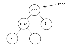
Functional program in tree representation

This program simply takes the maximum of 5 and whatever x is and then adds 2. In this example add and max are functions and x, 5 and 2 are terminals.

A functional program can also be written as an s-expression or parenthesized lists. A function call is then written as a list with the function name first and the arguments following. The example above as an s-expression becomes (add (max x 5) 2).

To solve a problem with GP, a set of functions and terminals must be defined that is appropriate to the problem to be solved. This is where specific domain knowledge comes in. Choosing the right function and terminals as well as defining the right fitness function can have a great impact on the performance of GP.

The creation of programs in GP heavily uses random factors. The first generation of programs is created randomly. Also the crossover and mutation operators that are used to create later generations use random numbers. This is to ensure that the search space (of all possible programs) gets explored thoroughly. However, the random creation of programs can lead to programs that make no sense at all or that can’t even be properly evaluated because a function argument doesn’t return the type of value that the function needs. To circumvent this problem strong typing is used. In Strongly Typed Genetic Programming[59] (STGP) a set of types is defined (suiting the problem domain) and every function and terminal is defined to return a specific type and every function argument is defined to be of a specific type. This defines which functions and terminals can be used as arguments for other functions. When done properly, strong typing can significantly help the creation of more meaningful and fitter programs.

III.2 Genetic programming in Adaptive Modeler

Adaptive Modeler uses a special adaptive form of strongly typed genetic programming. The genomes (programs) are the trading rules of agents. Their task is to trade the security on the Virtual Market based on their analysis of historical data. The fitness function is a measurement of an agent’s investment return over a certain period. However, there are some important differences between the way Adaptive Modeler uses (strongly typed) genetic programming and the general way described previously.

III.2.1 Main differences between Adaptive Modeler and conventional (strongly typed) genetic programming

In Adaptive Modeler, evaluating the fitness of agents does not involve any repeated hypothetical application of their trading rule on historical bars. This is because agents have already executed their trading rule on those historical bars once (on behalf of their role in the agent-based model) and Adaptive Modeler is only interested in the returns that they have already made “for real” in the agent-based model simulation, not in any theoretical returns that an agent could have made if it was sent back in time again.
In conventional GP, the programs are evaluated by the same fitness function every generation. For the purpose of Adaptive Modeler, a dynamic fitness function is needed. Every time the fitness of agents is evaluated, the return calculation period shifts forward to include the most recent quote bars. (In GP terms this could be called a kind of retraining method). Also, the process of creating new generations of agents in Adaptive Modeler has no termination criterion, since there is no fixed target fitness level to be achieved. As long as new market data keeps coming in, the population keeps evolving.
Adaptive Modeler normally doesn’t use the concept of generations as described earlier. Instead, a steady-state approach is used in which only a small part of the population is replaced at a time (typically every bar) instead of the entire population at once. This allows for a gradually changing population which is necessary to maintain a certain level of stability.

III.2.2 Input of the trading rules

The input of the trading rules can consist of the imported historical market data of the security, custom input variables if provided, and price and volume data from the Virtual Market. Also the agent’s current position in the security can be used as input. The actual input of the trading rules can be controlled by the gene selection.

III.2.3 Output of the trading rules

The output of the trading rules is an “Advice” consisting of a desired position in the security (as a percentage of wealth) and an order limit price or market order indication for buying or selling the security.

III.2.4 Defined types

The table below lists the types that have been defined for the implementation of strongly typed genetic programming in Adaptive Modeler. They are described in detail below the table.

Type	Description
Advice	Combination of a Position and a Limit (root type).
Position	Position in the security as % of wealth
Limit	Order limit price
Direction	Position direction (long, short or cash)
Leverage	Absolute position size as % of wealth
Quote	Price (from Real or Virtual Market data)
Volume	Volume (from Real or Virtual Market data)
Market	Real Market or Virtual Market
Change	Difference between two values (in %)
Lag	Number of bars
Bool	Boolean (True or False)
Custom	Value of a custom input variable
Digit	Numerical digit

III.2.4.1 Advice

This is the root type of the genome tree, meaning that the genome’s root node (which returns the final output of the trading rule) must be of this type. An Advice consists of combination of a Position value and a Limit value. They are combined (encoded) into an Advice value simply because a tree can have only one root node and thus return only one value.

III.2.4.2 Position

This type is used to denote the size and direction of an agent’s position (asset allocation) in the security as a percentage of its wealth. For instance, if an agent’s position is 100% then it owns only shares and no cash. Note that negative positions represent short positions.

III.2.4.3 Limit

This type is used for limit prices of agent orders or to indicate a market order. Arguably, the type Quote could have been used for this, but having a specific type for order limit prices allows more control over the way order limit prices are being generated.

III.2.4.4 Direction

This type is used to denote “position directions”. For this type only three possible values exist: long, short and cash (corresponding with the sign of a Position value). This type is used in combination with Leverage to create Position values.

III.2.4.5 Leverage

This type is used for an agent’s absolute position size as a percentage of wealth (in other words the Position without sign/direction). For instance a leverage of 50% means an agent has a position of 50% of its wealth in the security, either long or short. This type is used in combination with Direction to create Position values.

III.2.4.6 Quote

This type is used for security prices, either from the Real or Virtual Market. It is used for open, high, low, close, bid or ask prices. It is also used for prices that were calculated as averages, maximum, minimum, etc.

III.2.4.7 Volume

This type is used for volume data, either from the Real or Virtual Market. It is also used for volume data calculated as averages, maximum, minimum, etc.

III.2.4.8 Market

This type denotes the market type. Only two values of this type exist: Real Market and Virtual Market. This type is used for a market argument of several functions that can operate on either Real Market or Virtual Market data.

III.2.4.9 Change

This type is used for relative changes between two Quote values, two Volume values or two Custom values, for example a price change (return) such as p_t / p_t-1 - 1. It is also used for the agent’s breeding fitness return, given by the “Return” gene.

III.2.4.10 Lag

This type is used to denote a number of bars.

III.2.4.11 Boolean

This type is used for the boolean values True or False.

III.2.4.12 Custom

This type is used for values of a custom input variable. It is also used for custom input variable values calculated as averages, maximum, minimum, etc.

III.2.4.13 Digit

This type is used to represent numerical digits (0…9). One or more Digit values can be used to form numbers. For example this is used to denote the number of the custom input variable to be used by genes that use custom input variable data from the quote file.

III.2.5 Function and terminal set

In Adaptive Modeler, the function and terminals are also called “genes”. The entire set of genes with their return type and argument types is shown in the table below[60]. The terminals (with no arguments) have names starting with a capital and are listed on top. The functions follow below the terminals. Note that some functions (i.e. “+”, “>” and “if”) are defined more than once for different argument types and therefore have an (abbreviated) type suffix at the end of their name to distinguish them. The genes are described in more detail below the table.

Gene	Return type	Arg1 type	Arg2 type	Arg3 type	Arg4 type
CurPos	Position
Return	Change
LevUnit	Leverage
FullLev	Leverage
Rmarket	Market
Vmarket	Market
Long	Direction
Short	Direction
Cash	Direction
Bar	Lag
InvPos	Position
RndPos	Position
RndLim	Limit
MktOrder	Limit
IsMon	Bool
IsTue	Bool
IsWed	Bool
IsThu	Bool
IsFri	Bool
Digit0	Digit
Digit1	Digit
Digit2	Digit
Digit3	Digit
Digit4	Digit
Digit5	Digit
Digit6	Digit
Digit7	Digit
Digit8	Digit
Digit9	Digit
EMA10	Quote
EMA20	Quote
EMA50	Quote
EMA100	Quote
EMA200	Quote
open	Quote	Lag	Market
high	Quote	Lag	Market
low	Quote	Lag	Market
close	Quote	Lag	Market
bid	Quote	Lag	Market
ask	Quote	Lag	Market
average	Quote	Lag	Market
min	Quote	Lag	Market
max	Quote	Lag	Market
volume	Volume	Lag	Market
avgvol	Volume	Lag	Market
minvol	Volume	Lag	Market
maxvol	Volume	Lag	Market
custom	Custom	Lag	Digit	Digit
avgcustom	Custom	Lag	Digit	Digit
mincustom	Custom	Lag	Digit	Digit
maxcustom	Custom	Lag	Digit	Digit
>_quote	Bool	Quote	Quote
>_volume	Bool	Volume	Volume
>_custom	Bool	Custom	Custom
>_change	Bool	Change	Change
spread	Change	Market
barrange	Change	Lag
change_qt	Change	Quote	Quote
change_vo	Change	Volume	Volume
change_cu	Change	Custom	Custom
+_lag	Lag	Lag	Lag
+_lev	Leverage	Leverage	Leverage
*	Change	Change	Lag	Direction
dir	Bool	Lag	Market
isupbar	Bool	Lag	Market
upbars	Bool	Lag	Lag	Market
bsmin	Lag	Lag	Market
bsmax	Lag	Lag	Market
volat	Change	Lag	Market
rsi>=80	Bool	Lag	Market
rsi<=20	Bool	Lag	Market
sk>sd	Bool	Lag	Market
sk<sd	Bool	Lag	Market
ema	Quote	Lag	Market
mfi>=80	Bool	Lag	Market
mfi<=20	Bool	Lag	Market
pos	Position	Direction	Leverage
addpos	Position	Direction	Leverage
lim	Limit	Quote	Quote	Lag	Direction
mrlim	Limit	Market	Lag
tflim	Limit	Market	Lag
advice	Advice	Position	Limit
and	Bool	Bool	Bool
or	Bool	Bool	Bool
not	Bool	Bool
if_quote	Quote	Bool	Quote	Quote
if_lag	Lag	Bool	Lag	Lag
if_change	Change	Bool	Change	Change
if_bool	Bool	Bool	Bool	Bool
if_advice	Advice	Bool	Advice	Advice
if_market	Market	Bool	Market	Market
if_dir	Direction	Bool	Direction	Direction
if_limit	Limit	Bool	Limit	Limit
if_lev	Leverage	Bool	Leverage	Leverage
if_pos	Position	Bool	Position	Position
if_volume	Volume	Bool	Volume	Volume
if_custom	Custom	Bool	Custom	Custom

III.2.5.1 CurPos

CurPos returns the agent’s current position in the security as a percentage of its wealth (i.e. 100% is a full long position, 0% is a cash position and -100% is a short position for 100% of wealth). This gene is used for enabling agent to keep their current position.

III.2.5.2 Return

This gene gives the agent’s Breeding Fitness Return. The idea behind this is to give agents some reflexivity by letting them observe their own trading performance. This is based on the assumption that the behavior of market participants is affected by their own (recent) returns. This gene should be combined with other genes of type Change such as “change_qt”, “volat” and “*”.

III.2.5.3 LevUnit

LevUnit is the minimum increment (stepsize) of leverage (the absolute position size as % of wealth). During model evolution it is a constant value that is specified by the “Minimum position increment” setting on the “Model” tab of the “Model Configuration” dialog box. Leverage values can be added (by the “+_lev” gene) to create larger leverage values.

III.2.5.4 FullLev

FullLev is a constant value of 100% representing “full leverage”. This gene can be used instead of the “LevUnit” and “+_lev” genes to force agents to only place orders for 100%, -100%, or 0% positions. Using only this gene will result in shorter genomes since no repeated “+_lev” operations will be needed to reach higher leverage values. Shorter genomes may increase computation performance and are easier to read.

III.2.5.5 Rmarket, Vmarket

Indicates the Real Market (the imported security price and volume data) or the Virtual Market (the price and volume data of the Virtual Market).

III.2.5.6 Long, Short, Cash

Indicates a long, short or cash position direction (constant value of 1, -1 or 0). These terminals are used in for instance the “pos” function to create a Position by multiplying a Leverage value with a Direction value.

III.2.5.7 Bar

Indicates a single bar (constant value of 1). This terminal is used to create Lag values that are used to indicate a period length (in number of bars) for retrieving historical market data or calculating indicators such as average. Lag values can be added (by the “+_lag” gene) to create larger Lag values. (Note that Lag values are always at least 1).

III.2.5.8 InvPos

InvPos returns the opposite position of the agent's current position by multiplying the current position with -1 (long becomes short and vice versa).

III.2.5.9 RndPos

Returns a random position value ranging from -100% to 100% sampled from a uniform distribution. This gene can be used to simulate zero-intelligence agents.

III.2.5.10 RndLim

Returns a random limit price that is generated as follows. First the Virtual or Real Market is chosen at random. Then the last close price is taken from this market. Then this price is multiplied with a normally distributed random value with μ=1 and σ=3.5*σ_mwhere σ_mis the standard deviation of the log returns of the last 50 bars of the chosen market[61]. This gene can be used to simulate zero-intelligence agents.

III.2.5.11 MktOrder

Indicates that an order should be placed as a market order.

III.2.5.12 IsMon, IsTue, IsWed, IsThu, IsFri

These are Boolean functions that indicate whether or not the last bar (the bar before the current bar) is a Monday, Tuesday, Wednesday, Thursday or Friday.

III.2.5.13 Digit0, …, Digit9

These genes return the constant values 0 to 9. One or more of these genes can be used to form numbers. For example, this is used to form the number of the custom input variable to be used by genes that use custom input variable data from the quote file.

III.2.5.14 EMA10, …, EMA200

These genes return an exponential moving average of the closing price over the last 10, 20, 50, 100 or 200 bars on the Real Market. So in contrast to the non-terminal ema gene that has arguments for the period length and the market, these genes are terminals and use fixed period lengths and only operate on the Real Market. The period lengths of 10, 20, 50, 100 and 200 have been chosen because they are some of the most widely used periods for calculating exponential moving averages.

III.2.5.15 open, high, low, close

These functions return price data from the Real or Virtual Market. As arguments they take a Lag value for specifying which historical bar to use and a Market value for specifying either the Real or the Virtual Market. For instance, close(l,m) returns the close price of bar t-l on market m, where t is the current bar. For the Real Market, if open, high or low prices are not included in the quote file, the close price is returned. For the Virtual Market, open, high and low always return the close price (the clearing price). (Note that since a Lag value is always at least one, only bars before the current bar can be requested. This is because at the time the genomes are being evaluated, the current bar number already points to the bar being forecasted for which the Real Market data is still unavailable. Therefore at the time of genome evaluation, the bar before the current bar always has the most recent Real Market data).

III.2.5.16 bid, ask

Bid and ask return the bid and ask price data for the specified bar and market. For the Real Market, the bid and ask prices from the quote file are returned. If the bid or ask prices are not included in the quote file or if they are 0, then the close price is returned. For the Virtual Market, the bid and ask price are returned as defined in VM Bid and Ask.

III.2.5.17 average, min, max

These functions calculate the average, minimum or maximum of the close prices over the last given number of bars on the given market. For example, average(l,m) is the average close price over bars [t-l,t-1] on market m, where t is the current bar. Note that the high and low price data is not used in the calculation of min and max.

III.2.5.18 volume

Returns volume data for the specified bar and market. For the Real Market this is the volume data included in the quote file. If no volume data is included in the quote file while this gene is selected, this function returns 0. For the Virtual Market the volume data is defined as in VM Volume.

III.2.5.19 avgvol, minvol, maxvol

These functions calculate the average, minimum or maximum volume over the last given number of bars on the given market. For example, avgvol(l,m) is average volume over bars [t-l,t-1] on market m, where t is the current bar.

III.2.5.20 custom

Returns the value of a custom input variable for the specified bar. The number of the custom input variable to use is indicated by two Digit arguments. Specifically, custom(l,d1,d2) returns the value of custom input variable i at bar t-l, where t is the current bar and i is calculated as (d1 * 10 + d2) mod n, where n is the number of custom input variables in the quote file. Because of the modulo operator, every combination of Digit arguments will be valid. Because two Digit arguments are used, up to 100 custom variables can be indicated if all Digit genes are enabled. Note that when only one custom variable is included in the quote file, only one Digit gene needs to be enabled in the gene selection (and it doesn’t matter which one). When multiple custom input variables are included in the quote file, more (or simply all) Digit genes need to be enabled. If no custom input variable is included in the quote file then this function always returns 0.

III.2.5.21 avgcustom, mincustom, maxcustom

These functions calculate the average, minimum or maximum value of a custom input variable over the last given number of bars. For example, avgcustom(l,d1,d2) returns the average value of custom input variable i over bars [t-l,t-1], where t is the current bar and i is calculated in the same way as for the custom gene.

III.2.5.22 >_quote, >_volume, >_custom, >_change

The “>” functions are greater than comparisons for argument pairs of the types Quote, Volume, Custom or Change. It returns True if the value of the first argument is greater than the value of the second argument, False otherwise. Note that “<” functions are not defined nor necessary since the arguments can appear in either order. Also no “>=” or “=” functions are defined since they are logically equivalent to “not <” resp. “not > and not <”.

III.2.5.23 spread

Returns the spread of the last bar (t-1) on the specified market. The spread is expressed as a percentage of the close price and is therefore calculated as (ask – bid) / close. If the bid or ask price is 0 or not available then this function returns 0.

III.2.5.24 barrange

This function returns the high/low range of the specified bar on the Real Market. The high/low bar range is calculated as (high - low) / close.

III.2.5.25 change_qt, change_vo, change_cu

The “change” functions are defined for argument pairs of the types Quote, Volume or Custom. It returns the relative change of the first argument value from the second argument value. For instance, change_qt(q1,q2) returns q1/q2 – 1. In case the second argument value is zero, this function returns zero.

III.2.5.26 +_lag, +_lev

The “+” functions are defined for argument pairs of the types Lag and Leverage. It simply adds Lag or Leverage values to create larger values from smaller ones.

III.2.5.27 *

The “*” function multiplies a Change value with a Lag and Direction. This may be useful to multiply volatility values i.e. to create Bollinger Band like functions and to enable wider use of Change values in general.

III.2.5.28 dir

This function calculates the price direction over the last specified number of bars on the given market and returns a boolean value to indicate whether or not the direction is upwards. More specifically, dir(l,m) returns True if close(t-1,m) > close(t-1-l,m), where t is the current bar.

III.2.5.29 isupbar

Returns a boolean value to indicate whether the specified bar on the specified market is an “up” bar or not. More specifically, isupbar(l,m) returns True if close(t-l,m) > close(t-l-1,m), where t is the current bar.

III.2.5.30 upbars

This function checks if the number of “up” bars during the last specified number of bars on a given market is higher than or equal to a given number. More specifically, upbars(l1,l2,m) returns True if the number of up bars on market m during [t-l1,t-1] >= l2, where t is the current bar.

III.2.5.31 bsmin, bsmax

These functions stand for “bars since minumum” and “bars since maximum”. They return the number of bars since the minimum/maximum close price over a given period. For example, bsmin(l,m) returns the number of bars since the minimum close price over bars [t-l,t-1] on market m, where t is the current bar.

III.2.5.32 volat

This function returns the volatility (standard deviation) of the logarithmic returns of the close prices during the given period on the given market. For given arguments l and m, volat(l,m) returns the standard deviation of the most recent n bars on market m where n = l + 9. Since l is always at least 1, n is always at least 10.

III.2.5.33 rsi>=80, rsi<=20

These functions calculate an RSI (Relative Strength Index) value of the price data of the given period and market and return a boolean to indicate whether or not the value is higher than or equal to 80 resp. lower than or equal to 20. For given arguments l and m, the RSI is calculated over the most recent n bars on market m where n = l + 9. Since l is always at least 1, n is always at least 10.

III.2.5.34 sk>sd, sk<sd

These functions calculate a Stochastic Oscillator of the price data of the given period and market and return a boolean indicating whether or not the fast %K signal is higher (resp. lower) than the slow %D signal. For given arguments l and m, the Stochastic Oscillator is calculated over the most recent n bars on market m where n = l + 9. Since l is always at least 1, n is always at least 10. For example, sk>sd(l,m) returns True if the fast %K signal is higher than the slow %D signal over bars [t-l,t-1] on market m, and False otherwise.

III.2.5.35 ema

This function returns an exponential moving average of the price data of the given period and market. For given arguments l and m, ema(l,m) returns an exponential moving average of the most recent n bars on market m where n = l + 9. Since l is always at least 1, n is always at least 10.

III.2.5.36 mfi>=80, mfi<=20

These functions calculate an MFI (Money Flow Index) value of the volume data of the given period and market and return a boolean to indicate whether or not the value is higher than or equal to 80 resp. lower than or equal to 20. For given arguments l and m, the MFI is calculated over the most recent n bars on market m where n = l + 9. Since l is always at least 1, n is always at least 10. Note that the MFI calculation uses volume data and for the Real Market also high and low prices. If the volume data on the given market is zero during the calculation period, both MFI functions will return False. If high and low prices are not included in the quote file they will be considered equal to the close price.

III.2.5.37 pos

This function combines a Direction and a Leverage value into a Position. To do this it simply multiplies the Direction value with the Leverage value.

III.2.5.38 addpos

This function combines the Direction and Leverage argument values into a Position (like “pos”) and then adds the agent's current position. The resulting Position is returned. Note that the returned position value can be higher or lower than the agent’s current position.

III.2.5.39 lim

This function provides a simple model for calculating an order limit price. It takes as arguments two Quotes, a Lag and a Direction. The model is based on the assumption that traders determine their order limit price (to a certain extent) based on the observed market prices and the magnitude of (recent) price changes. The function calculates the difference between the two given Quote values, processes this difference a bit further with the given Lag and Direction values and adds this to the first Quote value. The agent’s way of calculating its order limit price and the “urgency” of its order can thus be represented in the choice of Quote values and Lag and Direction values. Note that the Lag and Direction types are used here for their arithmetic convenience and not because of their meaning. More specifically, lim(q1,q2,l,d) = q1 + l * 0.1 * d * (q2 - q1). Note that when the Direction value is zero the function simply returns q1.

III.2.5.40 mrlim

This function generates a "mean-reverting" order limit price[62]. It is based on the assumption that a trader uses a simple mean-reversion model to predict the next virtual market price, which it will use as its order limit price in the hope that its order will be executed in the next virtual market clearing, while minimizing price impact. The prediction can be based on either the Real Market prices or the Virtual Market prices, and assumes that the price will move toward its moving average. The moving average length is given by the Lag argument, increased by 1, so that it is always at least 2. Specifically, mrlim(m,l) = q + 2 * (ma - q)/(l+1) where q is the closing price of bar t-1 on market m and ma is the average closing price over bars [t-l-1,t-1] on market m, where t is the current bar.

III.2.5.41 tflim

This function generates a "trend-following" order limit price. It is based on the assumption that a trader uses a simple trend-following model to predict the next virtual market price, which it will use as its order limit price in the hope that its order will be executed in the next virtual market clearing, while minimizing price impact. The prediction can be based on either the Real Market prices or the Virtual Market prices, and assumes that the price will continue to follow its recent trend. The trend calculation period length is given by the Lag argument. Specifically, tflim(m,l) = q1 + (q1 - q2)/l where q1 is the closing price of bar t-1 on market m and q2 is the closing price of bar t-l-1 on market m, where t is the current bar.

III.2.5.42 advice

Combines a Position and a Limit value into an Advice. The Advice is ultimately returned by the genome (either directly through this function or through an “if_advice” function) and then processed further by the program as described in Order generation.

III.2.5.43 and, or, not

These are logical operators on their Bool arguments.

III.2.5.44 if_quote, if_lag, if_change, etc.

The “if” functions are defined for almost all types. The first argument is a Bool value. If this value is True, the second argument value is returned, otherwise the third argument value is returned.

[1] See for example: B. LeBaron, “Agent-based Financial Markets: Matching Stylized Facts with Style”, in Post Walrasian Macroeconomics: Beyond the DSGE Model, edited by D. Colander, Cambridge University Press, 2006: 221-235.

[2] See for example: Shu-Heng Chen, Chia-Ling Chang and Ye-Rong Du (2012), “Agent-based economic models and econometrics”. The Knowledge Engineering Review, 27, pp 187-219.
Or: Cars Hommes, “Heterogeneous Agent Models in Economics and Finance”, in Leigh Tesfatsion and Kenneth L. Judd (ed.), 2006. "Handbook of Computational Economics", Elsevier, edition 1, volume 2, number 2

[3] Values mentioned are upper limits. Actual values may depend on system configuration such as available memory and on specific model parameters and characteristics. See also 6.13 Computation performance issues.

[4] The Evaluation Edition processes recent quotes with a delay of a few days and thus delays forecasts and trading signals for the future. This prevents actual trading based on the trading signals. The Standard and Professional Editions do not have this limitation.

[8] Either the number of quote files or the number of models per security can be higher than 1 but not both. Neither value can be higher than 4. When entering information in the Batch Processing dialog these limitations will not be checked. When the batch is started they will be enforced however.

[9] Limited by available memory and system resources.

[10] Limited by available memory and system resources.

[11] To keep things simple, S&P500 index cash prices are used here instead of futures or ETF prices. Note that much more historical daily quotes exist for the S&P500 cash index than for SPY, which is useful for model evolution. Note that the included quote file does not contain open, high and low prices before 1962. They have therefore been set equal to the closing price.

[12] Actually, the first step is only a partial step. No new bar is read from the quote file yet since the bars before the model evolution start date are already in memory. The close price of the model evolution start bar will be forecasted but the “Bars processed” counter will stay at 0.

[13] The horizontal position of forecasts and signals in the chart is at the next bar. The vertical position of signals is at the last security close price.

[14] Adaptive Modeler uses scientific notation to show very large or small values (i.e. 1.00E+06 is 1 million).

[15] All return and performance indicators in Adaptive Modeler are calculated after all transaction costs (broker commissions, spread and slippage).

[16] Switching from a long to a short position or vice versa is counted as two transactions.

[17] Agent replacement may occur through regular breeding but also as a consequence of defaulted agents.

[18] If the same highest trading volume can be matched at multiple price levels, then the clearing price will be the average of the lowest and the highest of those prices. Market orders have no influence on the clearing price.

[19] Models using the same historical data, parameters and random seed may still vary with different versions of Adaptive Modeler. It may therefore not always be possible to recreate an earlier created model exactly with a new version of Adaptive Modeler. Models may possibly also vary across different computers because of small floating point calculation differences between different CPU types, Operating System versions and settings and .NET Framework runtime versions.

[20] Custom input variables are only supported in the Professional Edition.

[21] Effectively this means that the time needed for retrieving the quote and generating the forecast and signal should be no more than a fraction of the quote interval.

[22] With variable intervals, the periods shown in charts may not be exactly the same as the selected “Chart period” in the main toolbar.

[23] This is only supported in the Professional Edition.

[24] Since each bar must contain the same number of columns, an empty field must be indicated by a field delimiter. For example, if a custom input variable is in the last column, a row with no value specificied for the custom variable (empty field) should end with a comma (if comma is the field delimiter).

[25] When date and time are combined in one column, the exact date and time format can also be specified in the header, i.e. by “M/d/yy HH:mm:ss”.

[26] However, the bid and ask genes for the Real Market will return the Close price in case the Bid or Ask price is zero.

[27] A model is Adaptive Modeler’s main document type and contains all the data associated with the forecasting of a particular security including the state of the Agent-based Model, the Trading System, historical data and the model parameters.

[28] Incorrect Market Trading Hours will also cause more notifications in the Log.

[29] Reductions of trading hours will not be detected automatically.

[30] A. Dragulescu and V. M. Yakovenko, "Statistical mechanics of money", The European Physical Journal B, v. 17, pp. 723-729 (2000).

[31] A. Dragulescu and V. M. Yakovenko, "Exponential and power-law probability distributions of wealth and income in the United Kingdom and the United States", Physica A 299, 213-221 (2001).

[32] Nevertheless, some empirical studies (i.e. the one referred to in this paragraph) have shown wealth to be distributed exponentially as well.

[33] M. Matsumoto and T. Nishimura, "Mersenne Twister: A 623-dimensionally equidistributed uniform pseudorandom number generator", ACM Trans. on Modeling and Computer Simulation Vol. 8, No. 1, January pp.3-30 (1998).

[34] Also it is necessary to use the exact same historical quotes and model parameters and (in most cases) the same version of Adaptive Modeler. Models may possibly also vary across different computers because of small floating point calculation differences between different CPU types, Operating System versions and settings and .NET Framework runtime versions.

[35] The seed value of these random number generators is generated from the clock and can not be observed or set by the user.

[36] These values may be different than those that a running model is currently using. This allows testing other size and depth parameter values without disturbing the model. They will only become effective for the model if the user clicks “OK” or “Apply” in the “Model Configuration” dialog.

[37] This requires that the market’s opening time is set equal to the market’s closing time.

[38] In case the model contains more bars than the maximum number of bars that can be stored in memory, the chart will be scrolled back to the oldest bar in memory.

[39] The number of values indicates the number of values included in the distribution. Because some distribution series are related to agent characteristics that can not always be calculated for each agent (i.e. when an agent’s age is still too low), less values may be included than the population size.

[40] When too many bars are shown in the chart to locate every individual bar, the vertical position of the mouse can be used for fine tuning.

[41] The number of data points (bars) to show per chart period is calculated by assuming 5 trading days per week (i.e. as for stocks). For markets that also trade during the weekend, the periods effectively shown in charts will therefore be shorter since the number of bars per period is higher. Also when a variable quote interval is used, the periods effectively shown in charts may not be exactly as long as the selected chart period.

[42] The bin size (W) is automatically set according to W=3.49σN^-1/3 where σ is the standard deviation and N is the number of samples (D. Scott, “On Optimal and Data-Based Histograms”, Biometrika, Vol. 66, No. 3. Dec 1979, pp. 605-610). For the various distribution data series in Adaptive Modeler, this function generally gives the best histogram bin size with the most efficient, unbiased estimation of the probability density function. For data series that only return integer values (i.e. agent age) the bin size is rounded to ensure that bin edges coincide with integer values.

[45] The yellow bars do not necessarily represent all “matching” volume (volume of orders that will be executed at market clearing) because the book may also contain sell orders with an ask price below the bid price of a buy order. In this case these orders will be executed but won’t show up as yellow bars since the bid and ask prices are different.

[46] If no orders could be matched, no clearing price will be shown above the chart.

[47] Exceptions to this are caused by an imbalance in the total buy and sell volume.

[49] See for example: B. Qian, K. Rasheed, “Hurst Exponent and Financial Market Predictability”, IASTED conference on "Financial Engineering and Applications"(FEA 2004), pp. 203 – 209, 2004. The Hurst exponent chart for the Dow Jones in this paper can be exactly replicated with Adaptive Modeler.

[50] Receiver Operating Characteristic; a measure of the fraction of true positives versus the fraction of false positives. See for instance: T. Fawcett (2003), “Roc graphs: Notes and practical considerations for data mining researchers”, Technical Report HPL-2003-4. HP Laboratories.

[51] It should be noted that the concept of AUC is mostly associated with classifiers that return continuous values that are turned into binary classifiers by using a discrimination threshold. For such classifiers, a full ROC curve can be made through multiple (TPR, FPR) points by varying the discrimination threshold. Here however, the directional forecast is used as a binary classifier in itself without an adjustable threshold so only one (TPR, FPR) point exists. The calculation is therefore a “single point” AUC.

[54] Only when using MCS with a fixed starting capital and while leaving all Trading System parameters unchanged, the different outcomes per simulation are only being caused by random factors.

[55] This parameter now relates to the simulated “insignificant bars” that occur with probability 1-FDS instead of the “Significant Forecast Range” parameter which is not used by the Statistical Simulation data series.

[56] When “Generate cash signal at market close” is enabled, overnight returns will be excluded from the historical sampling period. So this effectively simulates that no overnight positions are being held. For continuous 24 markets such as Forex, only returns during the weekend will be excluded.

[57] Hurst, Simon R., Platen, Eckhard, “The marginal distributions of returns and volatility”, Statistical procedures and related topics, 301--314, Institute of Mathematical Statistics, Hayward, CA, 1997

[58] Kevin Fergusson, Eckhard Platen, “On the Distributional Characterization of Daily Log Returns of a World Stock Index”, Applied Mathematical Finance, Vol. 13, Iss. 1, 2006

[59] D.J. Montana, “Strongly typed genetic programming”, Evolutionary Computation 3(2), 199–230 (1995)

[60] Some genes are only included in the Professional Edition.

[61] This method is partly based on: M. Raberto, S. Cincotti, S.M. Focardi, M. Marchesi, "Agent-based simulation of a financial market", Physica A 299, 319-327 (2001). The difference is that here m=1 instead of 1.01 so that no spread is added/subtracted for increasing the likelihood of an order being executed. The reason for this is that in this implementation, at the time the RndLim gene is evaluated, it is not known whether the agent will place a buy or sell order and thus whether the spread should be added or subtracted.

[62] In the literature, many so called 2-type and 3-type agent-based models of financial markets distinguish a few different types of agents typically including fundamental traders (who belief the price will revert to the fundamental price), technical ‘momentum’ traders (trend-followers) and technical ‘contrarian’ traders (going against the trend). With respect to the expectation of the next virtual market price for use as the limit price, each of these types can essentially be represented by the mrlim and tflim genes, depending on the arguments being used. For an introduction into these models and further references, see: Shu-Heng Chen, Chia-Ling Chang and Ye-Rong Du (2012), “Agent-based economic models and econometrics”. The Knowledge Engineering Review, 27, pp 187-219.